What is the difference between sparse and dense embeddings?
Sparse and dense embeddings explained: what each representation is, how they differ in dimensionality, sparsity, indexing, and common use cases. Learn practical tradeoffs for search, storage, and interpretability so you can choose the right embedding type for a vector database problem.
TL;DR
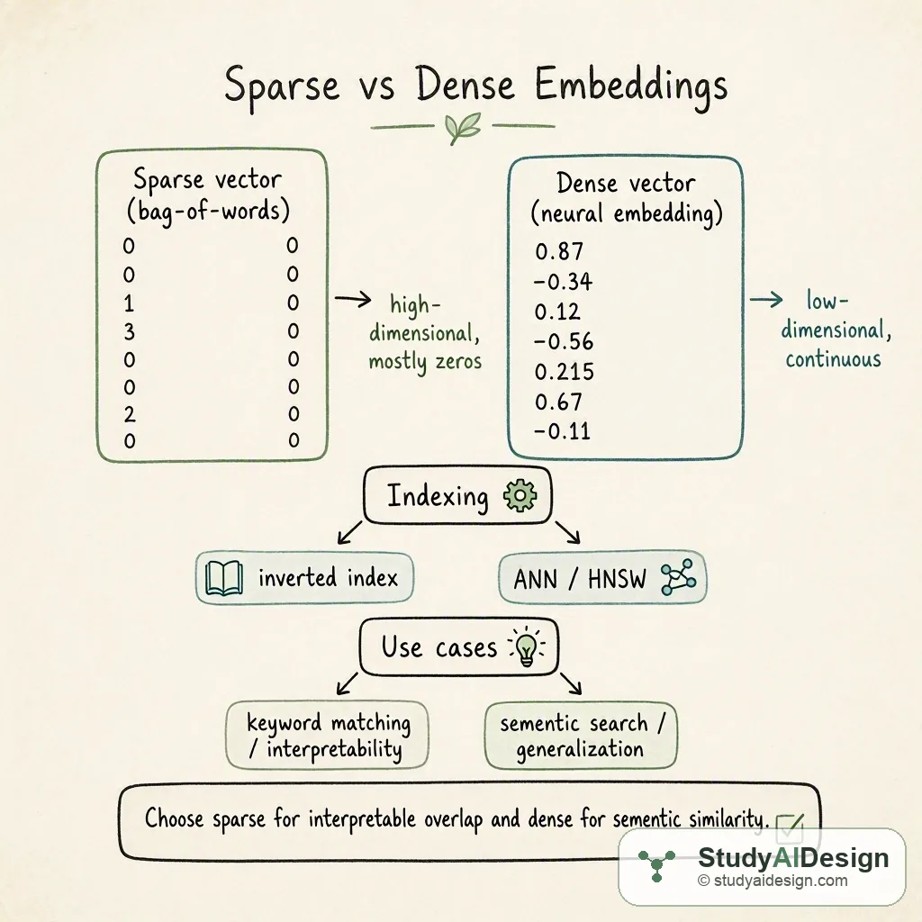
- Sparse embeddings are high dimensional and mostly zeros, derived from explicit token counts or weighted counts like TF-IDF.
- Dense embeddings are low dimensional, continuous vectors produced by neural models that capture semantic relationships.
- Sparse is cheap to index with inverted indexes and is interpretable; dense is compact, better for semantic similarity, and commonly used with ANN indexes. Key tradeoffs: interpretability and exact keyword overlap versus semantic generalization and compactness.
In this question, we will learn the core differences between sparse and dense embeddings and why those differences matter for vector databases and retrieval.
We will cover the following:
- The intuition
- How it actually works
- Indexing and search methods
- Tradeoffs and failure modes
- Questions the interviewer might ask
Direct answer: Sparse embeddings are high-dimensional, mostly-zero vectors built from explicit token counts or weighted counts and work well for keyword overlap and interpretability; dense embeddings are low-dimensional, continuous vectors learned by neural models and work well for semantic similarity and compact ANN search. Both can be used for retrieval, but they differ in dimensionality, storage, search algorithms, and failure modes.
The intuition (an analogy that makes it click)
Think of sparse embeddings like a library card catalog where each card marks presence or frequency of a specific term. Most cards are blank for a given book, so the representation has many zeros. That makes it easy to find documents that share exact words and to read why two items matched.
Dense embeddings are like fingerprints: each item gets a compact, continuous pattern that captures the overall shape of meaning. Two items with similar semantics have similar fingerprints even when they do not share exact words. You cannot read the fingerprint as easily, but it is great for matching by meaning.
How it actually works (the real mechanics)
Sparse embeddings
- Built from explicit features such as term counts, TF-IDF, or learned sparse encodings.
- Dimension equals vocabulary size or the number of features, often .
- Most coordinates are zero for any given document.
Dense embeddings
- Produced by neural encoders like transformers or sentence encoders.
- Dimension is usually small, e.g., , , or .
- Coordinates are real numbers and typically all nonzero.
Worked example: imagine two short documents and a small toy vocabulary.
Document A: "cat sat mat" Document B: "cat slept"
Vocabulary order: [cat, sat, slept, mat]
Sparse TF counts:
| term | cat | sat | slept | mat |
|---|---|---|---|---|
| A | 1 | 1 | 0 | 1 |
| B | 1 | 0 | 1 | 0 |
These become vectors in with many zeros for larger vocabularies.
Dense embeddings (toy):
| doc | dim1 | dim2 | dim3 |
|---|---|---|---|
| A | 0.6 | 0.1 | -0.2 |
| B | 0.58 | 0.05 | -0.25 |
Similarity measure: cosine similarity is common for both types. The formula is
For sparse vectors, the dot product counts overlapping terms and weights. For the toy sparse example, the dot product of A and B is because only "cat" overlaps. The norms reflect document lengths.
For dense vectors, the dot product and norms use the continuous coordinates; similar meaning produces higher cosine.
Comparison table (typical values):
| property | sparse | dense |
|---|---|---|
| dimension | to | to |
| typical nonzeros | small fraction | dense (most nonzero) |
| interpretability | high | low |
| best for | keyword overlap, explainability | semantic similarity, generalization |
| common index | inverted index | ANN (HNSW, IVF, PQ) |
Indexing and search
Sparse vectors map naturally to inverted indexes. Each nonzero feature points to a posting list of documents. Lookup for a query term touches only those postings, making exact keyword matching fast and explainable.
Dense vectors need approximate nearest neighbor search because linear scans over many dense vectors are expensive. Popular methods are HNSW, IVF+PQ, and product quantization. These accelerate cosine or inner product queries on compact vectors but introduce approximation.
A small comparison matrix:
| metric | inverted index (sparse) | ANN index (dense) |
|---|---|---|
| recall at scale | exact for matched terms | approximate, tunable via parameters |
| latency | predictable for term queries | sub-linear, depends on index settings |
| storage | can be large due to many feature positions | compact per vector but needs index structures |
When to choose which
- Use sparse embeddings when you need interpretability, exact keyword filtering, or when your signals are sparse by design, for example explicit tags or metadata.
- Use dense embeddings when you need semantic matching, retrieval across paraphrases, or you want compact storage and vector arithmetic for reranking.
You can also combine them: a common pattern is a hybrid retrieval pipeline where a sparse index handles high-precision keyword filters and a dense ANN index ranks semantically similar candidates.
Tradeoffs and failure modes
Sparse embeddings fail when documents use many synonyms or paraphrases because they rely on token overlap. They also explode in storage when the vocabulary becomes large.
Dense embeddings fail when domain shift makes the encoder misrepresent important tokens, or when you need clear explainability for legal or auditing reasons. ANN search can miss true nearest neighbors depending on tuning.
Questions the interviewer might ask
Some follow-up questions you might get:
How does TF-IDF relate to sparse embeddings? TF-IDF is a classic sparse embedding where each coordinate is term frequency times inverse document frequency. It emphasizes distinctive words and produces a high-dimensional sparse vector.
Why do we prefer cosine similarity for dense embeddings? Cosine focuses on angle rather than magnitude, which helps when vector magnitudes vary but direction encodes semantics. Inner product can work when vectors are length-normalized or when trained with that objective.
Can we compress sparse embeddings? Yes. You can use feature hashing or dimensionality reduction, but you may lose interpretability and exact matches. Learned sparse encoders can produce controlled sparsity.
What are hybrid retrieval pipelines? They combine sparse and dense retrieval stages. For example, start with a sparse inverted index to filter, then use dense ANN to rerank semantically similar candidates. This gives both precision and recall benefits.
How do you evaluate sparse vs dense retrieval quality? Use metrics like recall@k, MRR, and NDCG on labeled relevance sets. Compare latency and storage too, as practical constraints matter.
Some things to note:
- Calibration is important when combining scores from different spaces.
- Domain-specific finetuning of dense encoders often yields large gains.
What the interviewer is really testing
They want to see that you understand how representation choices affect retrieval architecture, performance, and explainability. They also want to hear practical tradeoffs: indexing method, storage implications, and how to combine signals. Show you can reason about both algorithmic and system-level consequences when choosing sparse or dense embeddings.
Further reading in the curriculum
Go deeper on the fundamentals behind this question.
- RAG Fundamentals Why retrieval-augmented generation works, and how to build a pipeline that actually grounds answers.
- Memory and State How AI systems store, retrieve, and manage information across tiers, from the context window to persistent knowledge stores.
Related questions
How would you rate the quality of this article?
Prepare for your AI engineering interview
This is one of many detailed questions and explainers on StudyAIDesign. Browse the full set, work through the curriculum, and walk into your interview ready.