training and adaptation
Part of the AI system design curriculum
Fine-Tuning and Adaptation
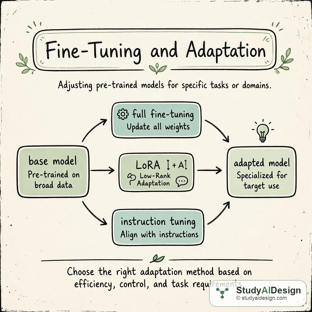
How to adapt pretrained language models to specific tasks using full fine-tuning, LoRA, instruction tuning, and preference alignment, and when each approach is the right tool.
TL;DR
- Fine-tuning is for changing model behavior, tone, or output format. Use RAG to add knowledge and facts.
- LoRA and QLoRA reduce memory requirements dramatically. They let you train large models on standard hardware by only updating a tiny fraction of the parameters.
- Data quality beats data quantity in instruction tuning. A thousand expert reviewed examples will outperform a hundred thousand scraped examples.
- Direct Preference Optimization (DPO) provides a simpler alternative to RLHF by eliminating the need to train a separate reward model.
- Full fine-tuning risks catastrophic forgetting, where the model loses its general capabilities. Parameter-efficient methods and data mixing prevent this.
A pretrained language model is a general-purpose reasoning engine: it can write, infer, and summarize across thousands of domains, but it does not know your product terminology, cannot reliably emit structured JSON, and will not match the tone your brand team spent months establishing. Fine-tuning takes that general engine and steers it toward a specific behavior, format, or domain. Done carefully, it cuts inference cost, shrinks prompt length, and outperforms even the most elaborate few-shot prompts. Done carelessly, it destroys the broad capabilities the base model spent hundreds of billions of compute tokens building. This chapter covers when to fine-tune, how the major techniques work, what can go wrong, and how to measure whether the investment was worth it.
When to Fine-Tune
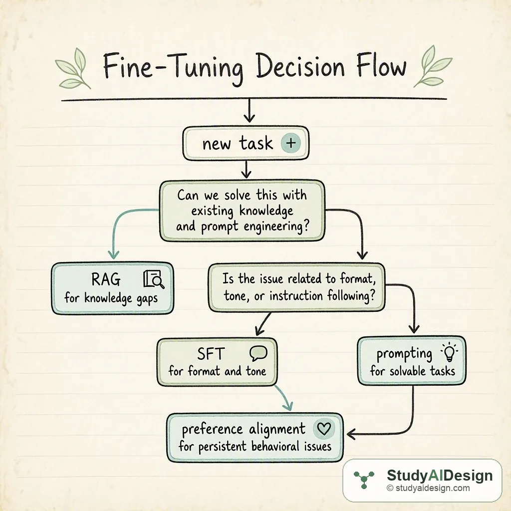
The most common mistake teams make is reaching for fine-tuning when the problem actually belongs to prompt engineering or retrieval. The three approaches solve different problems, and choosing the wrong one wastes weeks and produces worse results than the simpler option.
Prompt engineering is always the cheapest first move. A well-crafted system prompt with two or three high-quality examples costs nothing beyond a few hours of iteration. It fails when the task demands consistent structural output at scale, when few-shot context balloons prompts to 2,000 tokens or more, or when the base model simply lacks the behavioral pattern you need regardless of how you ask.
Retrieval-Augmented Generation is the right answer when the core problem is a knowledge gap. Models are poor at absorbing specific facts through fine-tuning: you would need each fact to appear in training many times before the weight updates encode it reliably, and even then the encoding degrades with distance from training distribution. An external index updated by a nightly re-index pipeline is simpler, cheaper, and always current. If the problem is "the model does not know about this document," the answer is retrieval, not training.
Fine-tuning is the right answer when the model needs to change its behavior, not expand its knowledge. Consistent JSON schema output, a specific persona, a compressed version of a few-shot pattern burned into weights to save context, or alignment to a set of human preferences are all genuine fine-tuning use cases.
| Signal | Recommended approach |
|---|---|
| Model lacks a specific fact | RAG or continued pretraining |
| Inconsistent output format (JSON, XML) | Fine-tuning (SFT) |
| Wrong tone or persona | Fine-tuning (SFT) |
| Few-shot prompt is too long or costly | Fine-tuning (compress shots into weights) |
| Private domain vocabulary and syntax | Continued pretraining, then SFT |
| Model gives harmful or off-policy responses | Preference alignment (DPO or RLHF) |
| Need a smaller model with large-model quality | Knowledge distillation |
Full Fine-Tuning
Full fine-tuning updates every parameter in the model on your task-specific dataset. The optimizer computes gradients across all weights, which means GPU memory must hold the model weights, all gradient tensors, and optimizer states simultaneously. For a 7B parameter model in 16-bit mixed precision under AdamW, that is approximately 7 billion parameters times 16 bytes (weights at 2 bytes, gradients at 2 bytes, and two optimizer state tensors at 4 bytes each), totaling around 112 GB of GPU memory. A single A100 80 GB cannot hold it. A 70B model requires roughly 1.1 TB, demanding many nodes with high-speed interconnects.
Beyond compute cost, full fine-tuning carries the highest risk of catastrophic forgetting. Weight updates push the entire parameter space toward your narrow dataset, and representations that supported general reasoning get overwritten by gradient steps that never saw those tasks.
Full fine-tuning is justified in three narrow situations: building a new foundation model from scratch, doing domain adaptation at scale with hundreds of billions of tokens of domain text (think training a dedicated biomedical or legal base model), or when parameter-efficient methods have already been exhausted and the quality gap is large enough to warrant the infrastructure. For product teams, it is almost never the right starting point.
Parameter-Efficient Fine-Tuning
Parameter-efficient fine-tuning (PEFT) methods update a small fraction of the model's parameters, typically under one percent, while freezing the rest. The quality improvement is nearly equivalent to full fine-tuning on most tasks, but the memory and compute cost is a fraction of the full approach.
LoRA: Low-Rank Adaptation
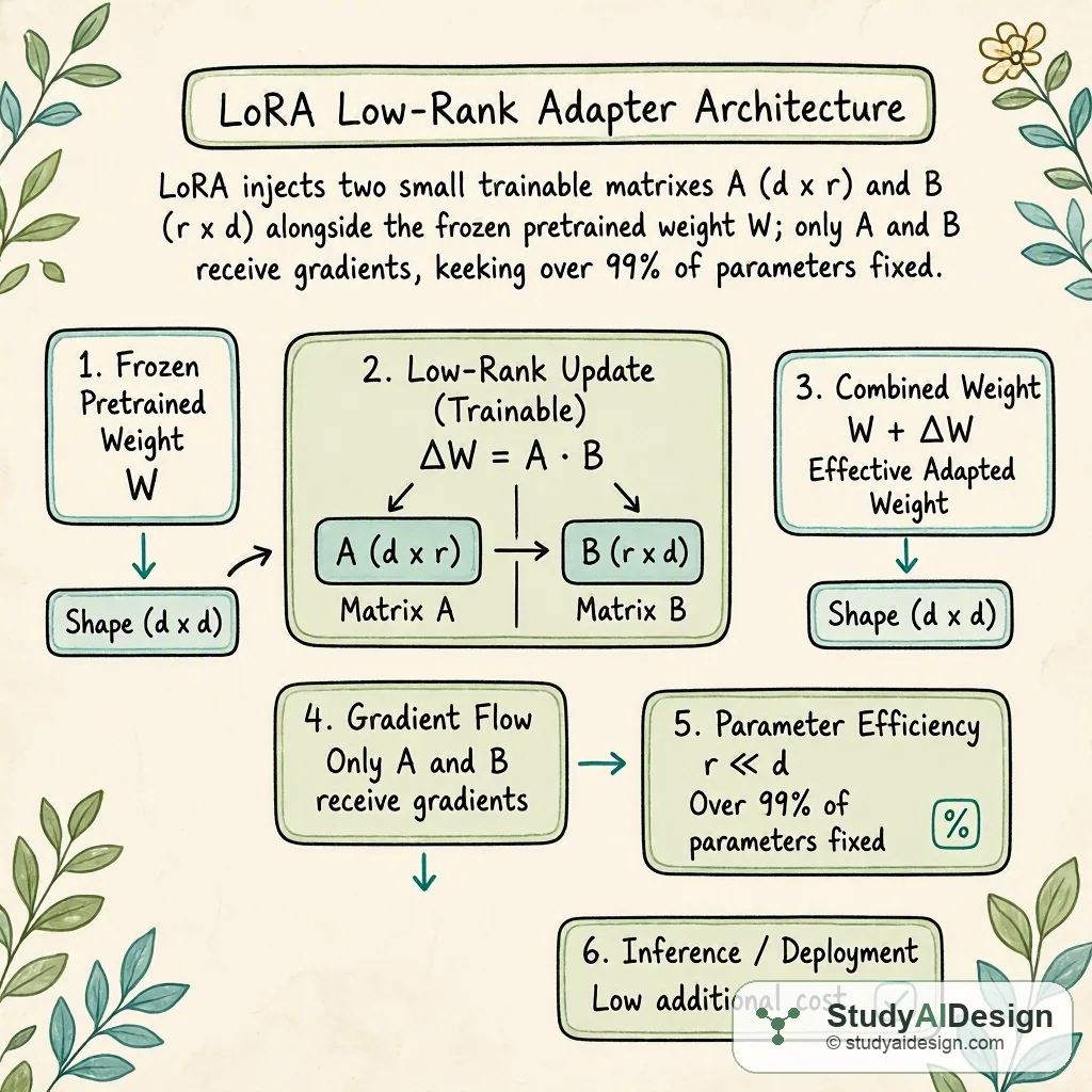
LoRA is the workhorse PEFT method. The core insight is that weight updates during fine-tuning tend to live in a low-dimensional subspace: even in a dense weight matrix W of shape d x d, most of the meaningful adaptation can be captured by a much smaller number of directions. LoRA exploits this by decomposing each weight update into two small matrices A (shape d x r) and B (shape r x d), where the rank r is much smaller than d.
The modified forward pass becomes:
h = Wx + (alpha / r) * BAx
Where W is the frozen pretrained weight, A is initialized with random Gaussian values, B is initialized to zero so the adapter contributes nothing at the start of training, and alpha is a scaling hyperparameter usually set to twice the rank. Only A and B receive gradients. W never changes.
For a 7B model with d = 4096 and r = 16, each LoRA adapter pair replaces a 4096 x 4096 = 16.7 million parameter update with two matrices totaling 4096 x 16 + 16 x 4096 = 131,072 parameters, a compression of roughly 128x. Applied to all linear layers, the total trainable parameter count lands between 0.1 and 1 percent of the base model.
Rank selection is the primary dial. Lower ranks (r = 4 to r = 16) handle simple behavioral changes like output format or persona. Higher ranks (r = 32 to r = 64) cover most domain adaptation tasks. Tasks requiring complex reasoning shifts may benefit from r = 128 or higher, though RS-LoRA's alpha / sqrt(r) scaling is recommended at those ranks to stabilize gradients. Start at r = 16, evaluate on your task metric, and only increase if the quality gap is measurable.
Target modules are the second dial. Early LoRA work applied adapters only to query and value projections in attention. Modern practice targets all linear layers: query, key, value, and output projections in attention, plus gate, up, and down projections in each MLP block. Broader targeting at a modest rank consistently outperforms narrow targeting at high rank.
QLoRA: 4-Bit Fine-Tuning
QLoRA extends LoRA by quantizing the frozen base model to 4-bit using NF4 (Normalized Float 4) before training begins. The LoRA adapters themselves remain in 16-bit precision. This reduces base model memory by roughly 4x compared to 16-bit loading, enabling a 70B model that would otherwise require around 140 GB to fit comfortably on two 80 GB A100s with room for adapters and optimizer states.
QLoRA adds three further optimizations: double quantization (quantizing the quantization constants themselves, saving around 0.5 GB), paged optimizers (spilling optimizer states to CPU RAM during memory spikes), and gradient checkpointing. The accuracy cost relative to full-precision LoRA is typically one to two percentage points on standard benchmarks, which is acceptable for most production deployments.
| Method | VRAM for 7B | VRAM for 70B | Trainable params | Forgetting risk |
|---|---|---|---|---|
| Full fine-tuning | ~112 GB | ~1.1 TB | 100% | High |
| LoRA (r=16, fp16) | ~28 GB | ~280 GB | ~0.5% | Low |
| QLoRA (r=16, 4-bit base) | ~12 GB | ~48 GB | ~0.5% | Low |
DoRA and Emerging Variants
DoRA (Weight-Decomposed Low-Rank Adaptation) decomposes the weight update into independent magnitude and direction components, similar to weight normalization. Because the two components are updated separately, DoRA converges faster than standard LoRA and more often matches full fine-tuning quality at the same rank where LoRA falls short. It is worth trying when you find that LoRA at rank 64 still leaves a noticeable gap compared to a full fine-tuning baseline.
Vera takes a different direction: it uses fixed random projection matrices shared across all layers and trains only a small per-layer scaling vector. This reduces adapter size by roughly 10x compared to LoRA, which matters for large-scale multi-adapter serving where you need hundreds of task-specific adapters on a single base model and adapter memory is the binding constraint.
Instruction Tuning
Instruction tuning is supervised fine-tuning on prompt-response pairs where the prompt is a natural language instruction and the response demonstrates the desired behavior. It is the step that converts a base model, which predicts the next token over raw text, into an assistant that follows directions. The training format is straightforward:
{
"prompt": "Summarize the following paragraph in one sentence:\n\n{paragraph}",
"response": "{summary}"
}Quality matters far more than quantity. A curated set of 1,000 diverse, expert-reviewed examples consistently outperforms 100,000 automatically scraped prompt-response pairs with inconsistent quality. Diversity is equally important: if all 10,000 examples are variations of the same three task types, the model generalizes poorly to anything outside that narrow distribution. Measure coverage by the breadth of distinct instruction categories, not raw example count.
Negative constraint training is an underused technique. Including examples of what the model should refuse or redirect, with the correct response as a label, teaches the model to handle off-policy requests gracefully rather than comply with harmful ones or produce an awkward non-answer. An explicit "I cannot help with that request" example is worth dozens of passive safety instructions embedded in a system prompt.
Learning rate matters more in instruction tuning than in pretraining. The standard range is 1e-5 to 5e-5 for SFT. Too high and the model collapses within the first few hundred steps, repeating tokens or producing incoherent output. Too low and training never escapes the pretraining distribution. Warm up the learning rate over the first 3 to 5 percent of steps, then use cosine decay.
Preference Alignment
Instruction tuning teaches a model to follow directions. Preference alignment teaches it to follow directions well, in the sense that humans reliably prefer its outputs over plausible alternatives. The input to alignment is a preference dataset: for each prompt, a "chosen" response that annotators preferred and a "rejected" response they did not.
RLHF
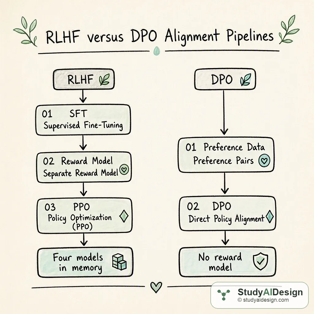
Reinforcement Learning from Human Feedback proceeds in three stages. First, an SFT model is trained as described above. Second, a separate reward model is trained on preference pairs to predict which response humans prefer: it takes a (prompt, response) pair as input and outputs a scalar score. Third, the SFT model is further optimized with Proximal Policy Optimization (PPO), using the reward model as a training signal, with a KL divergence penalty to prevent the policy from drifting too far from the SFT starting point.
RLHF is powerful but operationally demanding. PPO requires four models in memory at once: the policy being trained, a frozen reference policy for KL computation, the reward model, and the value model used by PPO to estimate expected returns. At 7B parameters and 16-bit precision, that is roughly 14 GB each, totaling around 56 GB before activations and optimizer states. PPO is also sensitive to hyperparameters and prone to reward hacking, where the policy learns to produce responses that score well on the reward model while being qualitatively unhelpful to actual users.
DPO: Direct Preference Optimization
DPO eliminates the reward model entirely. The insight from Rafailov et al. (2023) is that the optimal policy under the RLHF objective can be expressed analytically in terms of the preference data, which means you can optimize the policy directly on preference pairs without training a separate reward model.
The DPO loss is:
L = -log(sigmoid(beta * (log pi(chosen|x)/pi_ref(chosen|x) - log pi(rejected|x)/pi_ref(rejected|x))))
Where pi is the model being trained, pi_ref is the frozen reference model, and beta controls how strongly the policy is penalized for deviating from the reference. Training with DPO is as stable as classification: you only need the policy and the reference model in memory, and the optimization rarely exhibits the instabilities that make PPO difficult to tune.
One practical limitation of offline DPO is that it trains on a static preference dataset. Once the model's quality surpasses the quality ceiling in that dataset, it cannot improve further. Online DPO and RLOO address this by generating candidate responses at training time, scoring them with a judge model or a rule-based verifier, and constructing preference pairs dynamically from the model's own output. The tradeoff is additional complexity and compute: each training step now requires model inference in addition to gradient updates.
Knowledge Distillation
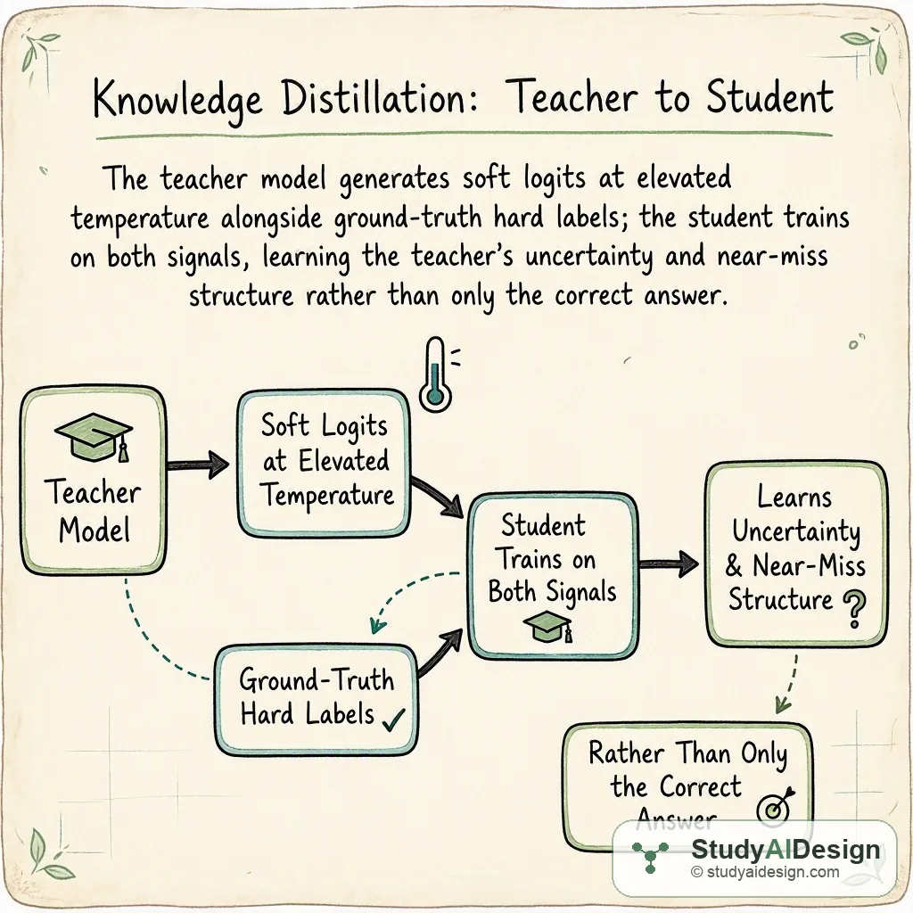
Knowledge distillation transfers the behavior of a large teacher model into a smaller student model. The student is trained not just to produce the same final answers as the teacher, but to match the teacher's full output distribution over all tokens. This richer signal, called soft labels, encodes not only which answer is correct but how plausible the alternatives were.
The distillation loss is a KL divergence between teacher and student distributions, computed at a temperature T:
# T = 2.0 to 5.0 softens the distribution, making near-misses visible
loss_soft = KL_div(softmax(teacher_logits / T), softmax(student_logits / T))
loss_hard = cross_entropy(student_logits, ground_truth_labels)
loss = alpha * loss_soft + (1 - alpha) * loss_hardAt T = 1 the soft loss collapses to standard cross-entropy on teacher predictions. At T = 2 to 5, the distribution is softened: if the teacher assigned 80% probability to "Paris" and 15% to "Lyon" for a question about France's capital, the student learns that Lyon was nearly correct, not just that Paris was right. This richer gradient signal accelerates convergence and tends to produce a student with better generalization than one trained on hard labels alone.
Self-distillation is how reasoning models improve without new human annotations. The model generates many candidate solutions to hard problems, a rule-based verifier (a test suite, a calculator, or a formal checker) identifies the correct ones, and the model is fine-tuned on the successful reasoning chains. The model curates its own training signal by filtering to only the chains that worked, then learns from those.
The main legal constraint: most commercial API providers explicitly prohibit using their outputs to train competing models. Distilling from GPT-4 or Claude via their APIs violates terms of service for most commercial use cases. Safe distillation pipelines use open-weight teacher models such as Llama 3 70B, Qwen 2.5 72B, or Mistral Large 2, all of which have licenses permitting downstream training.
Data Requirements and Failure Modes
How Much Data
For instruction tuning aimed at format changes or persona adjustments, 500 to 2,000 high-quality examples is often enough. For genuine domain adaptation across a wide variety of inputs, 10,000 to 50,000 examples is a more realistic floor. Preference alignment for DPO typically needs 5,000 to 20,000 preference pairs. RLHF requires more due to the added complexity of reward model training.
These figures assume high-quality data. Substantial noise, duplicates, or inconsistent quality push the required size up proportionally. The practical signal: if validation loss stops improving or diverges before training loss is competitive with human-level quality, the dataset is either too small or too noisy.
Catastrophic Forgetting
Catastrophic forgetting is the most common failure mode in full fine-tuning: the model's performance on tasks outside the fine-tuning distribution degrades, sometimes dramatically. The mechanism is direct. Gradient steps on a narrow dataset push all weights toward representations optimized for your training examples. Representations that supported unrelated tasks get overwritten because they never appear in the gradient signal.
Two mitigations work reliably. First, mix 5 to 10 percent of general pretraining data into the fine-tuning set. This forces continuous gradient reinforcement of general representations alongside the new task signal. Second, use LoRA or another PEFT method. Because the base model weights are frozen, the adapter optimization has no mechanism to damage the representations already in the pretrained weights. The catastrophic forgetting problem disappears structurally when the base is immutable.
Overfitting
Overfitting in LLM fine-tuning looks different from classical overfitting. The model may achieve low training loss and produce outputs that score well on automatic metrics, while generating repetitive, unnaturally short, or formulaic responses in practice. The cause is nearly always training too many epochs on too small a dataset: the model memorizes the training distribution rather than generalizing from it.
For most fine-tuning runs, one to three epochs is the right range. Beyond five epochs on a small dataset, quality regressions are almost guaranteed. Monitor this by reading actual model outputs, not just loss curves. A model scoring 0.95 on held-out validation loss but producing stiff, generic responses has overfit in a way that no automated metric catches.
Worked Example: SQL Generation with Llama 3 8B
A concrete scenario: a database analytics company wants a model that converts natural language questions into SQL queries for their internal schema. The base model (Llama 3 8B Instruct) achieves 52 percent execution accuracy on a held-out set of 500 labeled queries when prompted with the schema and three few-shot examples.
Dataset: 8,500 training examples, each consisting of a natural language question paired with a correct SQL query. Every query was validated by actually running it against the database and confirming the result. 500 examples held out for validation.
Method: QLoRA with r = 32, alpha = 64, targeting all linear layers. Base model quantized to 4-bit NF4. Training on a single A100 80 GB, learning rate 2e-4 with cosine decay, 3 epochs, batch size 4 with gradient accumulation of 8 steps (effective batch size 32). Total training time: approximately 4 hours.
| Variant | Execution accuracy | Avg prompt tokens | Relative inference cost |
|---|---|---|---|
| Base model + 3-shot prompt | 52% | 480 | 1.0x |
| Fine-tuned model + 0-shot | 76% | 120 | 0.25x |
| After second DPO pass | 81% | 120 | 0.25x |
The 0-shot fine-tuned model outperformed the 3-shot baseline by 24 percentage points and cut per-query inference cost by 75 percent by eliminating the few-shot context from every prompt. The DPO pass used 3,000 preference pairs, each constructed by comparing the fine-tuned model's output against the reference correct query and labeling pairs as chosen or rejected based on execution success.
A second training run with r = 8 achieved 71 percent accuracy at similar compute cost, confirming that rank 32 was meaningfully better than rank 8 for this task complexity. The accuracy gap between r = 8 and r = 32 (five percentage points) is enough to justify the modest additional memory overhead.
Interview Angle
Related Topics
How would you rate the quality of this article?
Keep going
Practice what you just read against real interview questions, or carry on through the curriculum.