model landscape
Part of the AI system design curriculum
Choosing the Right Model
A practical framework for navigating the 2026 model landscape and picking the right model for your use case, budget, and latency requirements.
TL;DR
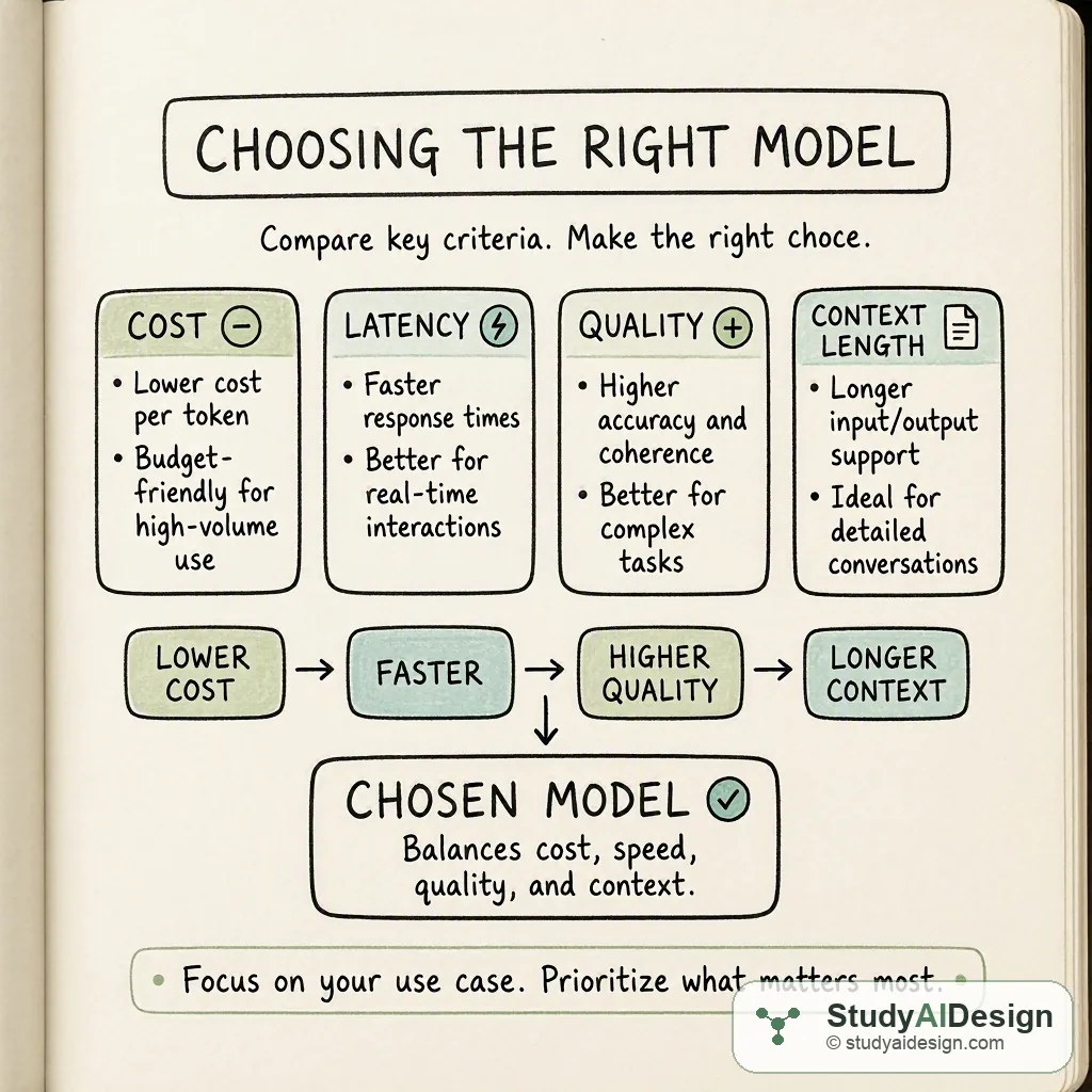
- Balancing capability, cost, and latency is the core of model selection. Frontier models excel at reasoning but are expensive and slow, while budget models are fast and cheap but struggle with multi-step tasks.
- Hosting open-weight models yourself only saves money if your GPU utilization is consistently high. Below 60 percent utilization, APIs are almost always the cheaper option.
- Implement multi-model routing to cut costs. Sending simple queries to budget models and saving frontier models for complex tasks can reduce your bill by up to 80 percent with minimal quality loss.
- Do not rely on public benchmarks for your final decision. Build a custom evaluation set of 100 to 200 real production queries to test how models actually perform on your specific workload.
The model landscape has quietly become one of the hardest engineering decisions in an AI system. Three years ago there were two or three credible API providers and the choice was simple. Today you are picking from dozens of models across four or five tiers, two access modes (hosted API versus self-hosted open weights), and a pricing structure that ranges from fractions of a cent to fifty dollars per million tokens. Pick the wrong model and you will either overpay by an order of magnitude or deploy something that fails quietly on the tail of your query distribution where it matters most.
The 2026 Model Landscape
Closed-Weight versus Open-Weight
The first axis that structures the landscape is not capability; it is access. Closed-weight models are served over an API by the provider. You send tokens, you get tokens back, you never see the weights. This is convenient and keeps operational costs low for teams without GPU infrastructure. The tradeoff is that data crosses the provider's network, you have no control over future price or availability changes, and you are bounded by the provider's rate limits and service agreement.
Open-weight models give you the weights under a license. You can run them on your own GPU cluster, an on-premises server, or a rented node, and your data never leaves your network. That privacy property is non-negotiable for healthcare, legal, and financial applications that carry strict data residency requirements. The operational cost is yours, however. Running a 70-billion-parameter model around the clock on dedicated hardware is cheaper than API calls only above a certain utilization threshold, typically around 60 to 70 percent GPU utilization. Below that, the reserved compute sits idle and the API is almost always cheaper.
Open weights do not mean free. A single H100 node on a major cloud provider costs roughly 0.40 to $0.60 per million tokens. That is competitive with mid-tier APIs only when throughput is steady and utilization is consistently high.
Model Families and Size Tiers
Within the closed-weight world, each provider runs a tiered family. Anthropic has Haiku (fast and cheap), Sonnet (balanced), and Opus (frontier). OpenAI runs mini, standard, and reasoning variants. Google has Flash, Pro, and Deep Think modes. The naming changes with every release cycle, but the underlying tiering logic is stable: small models handle high-volume simple tasks, mid-tier models cover the broad middle, and frontier models exist for tasks where capability ceiling matters more than cost.
Model size in parameters correlates with capability up to a point, but that correlation is loose in 2026. Mixture-of-Experts (MoE) architectures activate only a fraction of parameters per token. DeepSeek V4 Pro runs 671 billion total parameters but only 37 billion active parameters per forward pass, so the inference cost is closer to a 37B dense model while the capacity of the larger routing structure buys frontier-class reasoning. Size alone is no longer a reliable proxy for either cost or quality.
Context window is an increasingly important selection axis in its own right. Frontier models from Anthropic, OpenAI, and Google all support one-million-token contexts as of mid-2026. For corpora that fit comfortably under 100K tokens, long-context loading with prompt caching is often simpler than a full RAG pipeline, and pricing on cached tokens has dropped to 10 percent of standard input cost on Anthropic and OpenAI.
The Three-Way Tradeoff
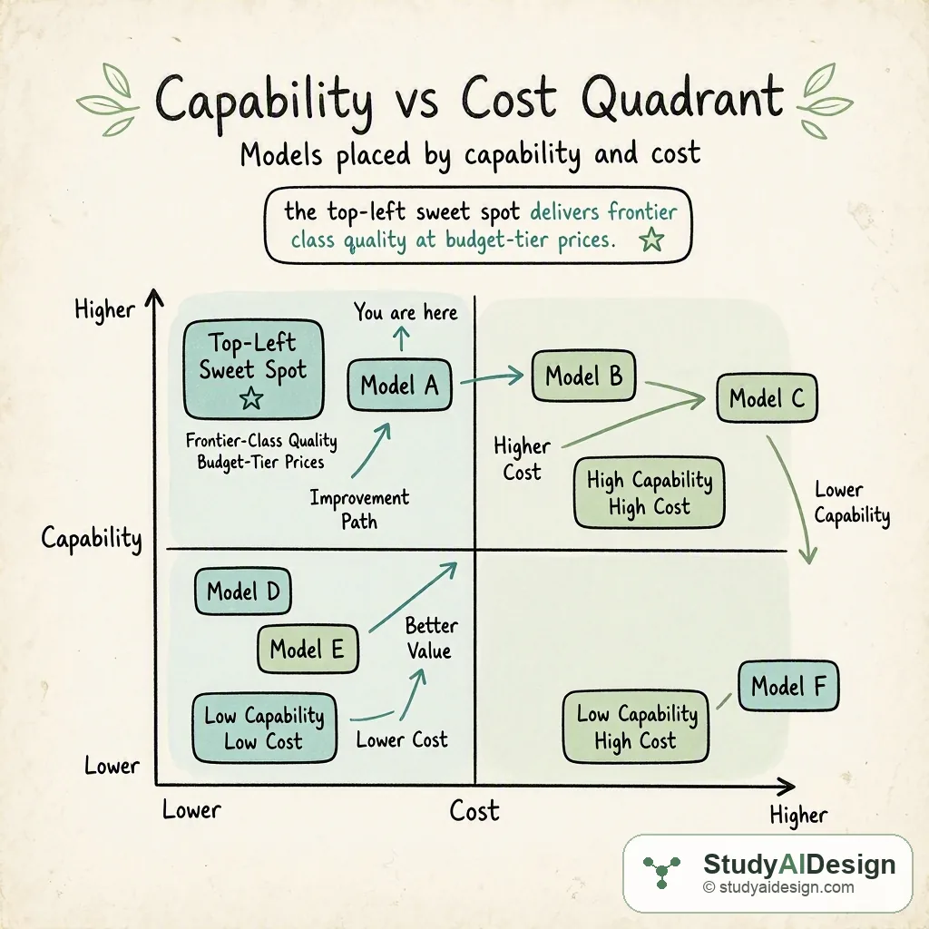
Every model selection decision lives inside a three-dimensional constraint: capability (what can it do well?), cost (what does it cost per token?), and latency (how fast does it respond?). These three dimensions pull in different directions, and optimizing for one almost always costs you in another.
Frontier models like Claude Fable 5 and Claude Opus 4.8 sit at the capability extreme. They handle multi-step reasoning, long-horizon agentic tasks, and difficult code generation with the best accuracy available. They also cost 50 per million input tokens and have median response times above one second under normal conditions. For a user-facing interface that must respond in under 200 milliseconds, they are simply the wrong tool regardless of their capability.
Budget models like Gemini 3.1 Flash (0.14) deliver sub-100 millisecond latency and are orders of magnitude cheaper at scale, but their reasoning depth drops off on complex multi-step tasks. Using them for agent orchestration or difficult code generation introduces silent failure modes: the model produces confident, plausible output that is wrong in ways that surface only during downstream validation.
The middle tier covers most production workloads. Models like Claude Sonnet 4.6 (2.00) are fast enough for interactive use, capable enough to handle 80 to 90 percent of real query distributions, and cheap enough that a million-query-per-month deployment costs 10,000 rather than $50,000.
A Model Selection Matrix
The table below captures current mid-2026 positioning across the tiers. Latency figures are median time-to-first-token estimates from US-East under typical load; actual production numbers vary by region and concurrent load.
| Model | Tier | Input $/1M | Output $/1M | Context | TTFT est. | Best For |
|---|---|---|---|---|---|---|
| Claude Fable 5 | Frontier | $10.00 | $50.00 | 1M | ~1.5s | Hardest reasoning, vision, long agents |
| Claude Opus 4.8 | Frontier | $5.00 | $25.00 | 1M | ~1.2s | Autonomous coding, agentic loops |
| GPT-5.5 | Frontier | $5.00 | $30.00 | 1M | ~1.0s | Single-shot coding, multimodal |
| Claude Sonnet 4.6 | Balanced | $3.00 | $15.00 | 1M | ~0.5s | General production workhorse |
| Gemini 3.1 Pro | Balanced | $2.00 | $12.00 | 1M | ~0.6s | Scientific reasoning, multimodal |
| DeepSeek V4 Pro | Balanced | $0.44 | $0.87 | 1M | ~0.7s | Lowest-cost frontier reasoning |
| GPT-5.5-mini | Budget | $0.75 | $4.50 | 272K | ~0.2s | High-volume chatbots, extraction |
| Gemini 3.1 Flash | Budget | $0.10 | $3.00 | 1M | ~0.15s | RAG at scale, real-time streaming |
| DeepSeek V4 Flash | Budget | $0.14 | $0.28 | 1M | ~0.12s | Cheapest frontier-class 1M context |
| Claude Haiku 4.5 | Budget | $0.25 | $1.25 | 200K | ~0.1s | Sub-100ms UI interactions |
| Llama 4 70B | Open-weight | self-hosted | self-hosted | 128K | hardware-dep. | On-prem, data residency |
TTFT = time to first token, estimated median. Verify on provider dashboards before sizing production infrastructure.
A Decision Framework
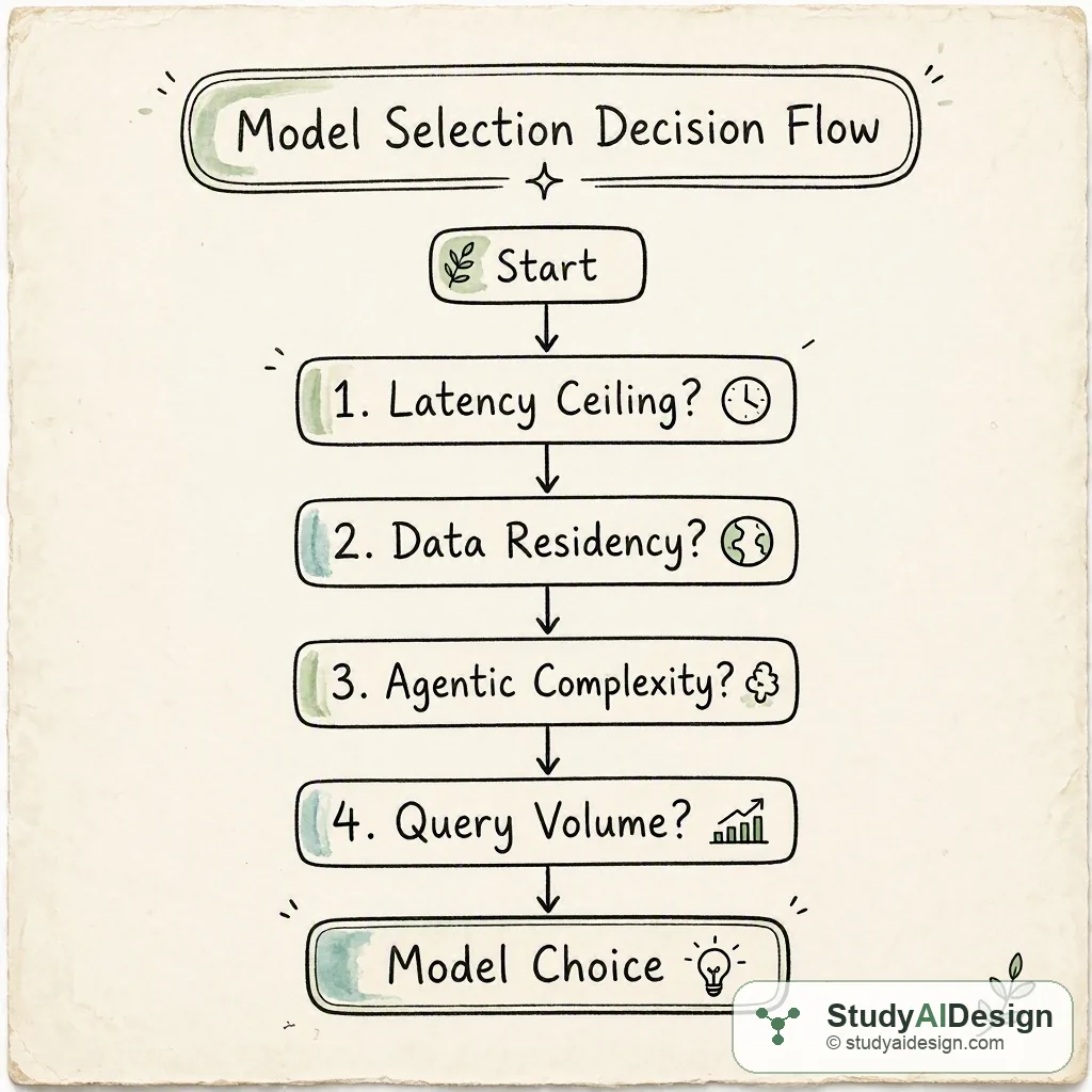
Before you open a pricing page, answer four questions in order. The first answer that fully resolves the problem ends the search.
Step 1: Does the use case have a hard latency ceiling? If the model must respond in under 150 milliseconds to keep a real-time interface feeling responsive, you are in the budget tier. Start with Gemini 3.1 Flash or Claude Haiku 4.5 and test whether quality is sufficient. If it is, the decision is over. If the task complexity pushes against quality limits at that tier, the only path forward is to redesign the interaction (pre-compute, cache, or handle asynchronously), because no frontier model hits 150ms reliably.
Step 2: Does data have to stay on-premises? If the answer must be yes, start with Llama 4 70B or DeepSeek V4 Pro on your own infrastructure. The operational cost and maintenance overhead are real. Do the GPU math before committing. If self-hosting is too expensive at current utilization, negotiate a data processing agreement with a closed-weight provider before deploying.
Step 3: Is this task agentic? Agentic tasks involving tool calling, multi-step planning, or autonomous execution over many turns have very different model requirements than single-shot generation. Tool-calling accuracy on frontier models (Fable 5, Opus 4.8, GPT-5.5) is substantially higher than on mid-tier or budget models. The failure mode for agentic workloads on under-powered models is silent: the agent produces plausible tool calls with subtly wrong parameters, and the error surfaces ten steps later as data corruption or a failed execution. For agentic work, start at Opus 4.8 and consider Fable 5 for the hardest orchestration tasks.
Step 4: What is the monthly query volume? For volumes below 100K queries per month, cost differences between tiers are rarely decisive; quality should drive selection. Above 1 million queries per month, a tier difference of 2,000 per month or $24,000 per year. Run the math. A mid-tier model is often adequate for 95 percent of the query distribution, with a smaller allocation of frontier-model calls handling the complex tail.
Multi-Model Routing
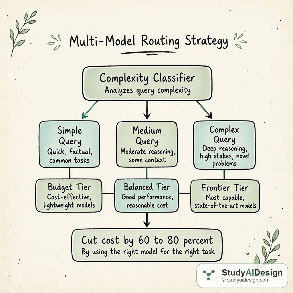
For high-volume systems, the answer to model selection is often not a single model but a routing strategy. A complexity classifier sits in front of the model tier, scores each incoming query, and routes accordingly:
- Simple queries (FAQ answers, entity extraction, classification) go to the budget tier
- Medium queries (summarization, structured output, moderate reasoning) go to the balanced tier
- Complex queries (code generation, multi-step analysis, agentic planning) go to the frontier tier
A well-calibrated router sends 60 to 70 percent of production traffic to the budget tier and only 5 to 10 percent to the frontier tier. The cost savings relative to routing everything to a frontier model are typically 60 to 80 percent, with minimal quality degradation on the majority of traffic. The classifier itself is usually a lightweight binary or three-class model trained on a few hundred labeled examples from your production query distribution; it does not need to be a frontier model.
Evaluating Before You Commit
Benchmarks and Their Limits
Public benchmarks like SWE-bench Verified, GPQA Diamond, and MMLU are useful for forming a rough prior about model tier, not for making final selection decisions. A model that ranks first on SWE-bench was evaluated on a specific distribution of GitHub issues, with a specific execution environment, under specific prompting conditions. Your task distribution almost certainly differs on all three dimensions.
The deeper problem with relying on public benchmarks is saturation. Models are frequently post-trained on benchmark-adjacent data, so high scores can reflect memorization rather than generalization. MMLU accuracy above 90 percent is now common across frontier models; the delta between 91 percent and 93 percent predicts nothing reliable about performance on a customer support transcript or a legal clause extraction task. When two models are separated by less than five percentage points on a public leaderboard, the benchmark is probably not the right signal for your selection decision.
Building Your Own Eval Set
The most actionable evaluation for model selection is a held-out sample of 100 to 200 real queries from your intended production distribution, labeled with expected outputs or quality ratings. Run each candidate model on this set and measure what matters for your use case: accuracy on your domain, format compliance, refusal rate on valid queries, latency at your actual prompt lengths, and cost per query.
Build your eval set before you select your model, not after. If you evaluate against a sample drawn from the same distribution you used to develop your prompts, you will overfit to one model's idiosyncrasies. A held-out set assembled before any prompt development is the only clean signal for comparison.
For a customer support use case, a useful eval set measures: correct answer rate (ground truth from previous agent-handled tickets), format compliance (does the response follow your specified structure?), and unnecessary refusal rate (does the model decline valid queries due to over-caution?). These three metrics reveal failure patterns that no public benchmark captures, and they can be computed on a few hundred examples in an afternoon.
Total Cost of Ownership
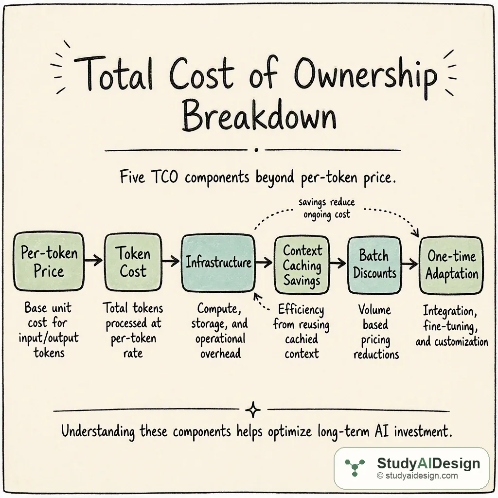
Per-token API price is the most visible cost but rarely the dominant one in production. Total cost of ownership (TCO) for a model deployment has several additional components.
Inference infrastructure and redundancy. Even with a hosted API, you need retry logic, fallback providers, and load balancing across regions. The engineering cost of building and maintaining a reliable inference layer is non-trivial. For self-hosted models, the GPU hardware, spot-instance risk, and DevOps overhead typically add 30 to 50 percent to the raw compute cost.
Context caching savings. If your system sends a long system prompt or a shared knowledge base on every request, context caching reduces input token cost by 80 to 90 percent on Anthropic and OpenAI models. A 10K-token system prompt sent to Claude Sonnet 4.6 for one million queries costs 3,000 with caching enabled. Failing to implement caching on a long shared prefix is a predictable and expensive mistake.
Batch API discounts. Both OpenAI and Anthropic offer 50 percent batch API discounts for requests that can tolerate 12 to 24 hour latency. Offline jobs such as document classification, data enrichment, or evaluation runs should use batch mode by default. Paying full real-time rates for async workloads is a common cost leak in production systems.
Fine-tuning and adaptation costs. If your use case requires a specialized model variant, add one-time training costs and ongoing serving costs for a private endpoint. Fine-tuning a 7B open-weight model on a domain corpus costs roughly 500 in GPU time; using a provider's hosted fine-tuning API costs significantly more. These are one-time costs that amortize quickly at scale but require upfront budget planning.
Worked Example: Customer Support at Scale
Consider a customer support system handling 500,000 queries per month. Average query: 800 input tokens (ticket text plus system prompt) and 300 output tokens (response). Requirements: sub-600ms TTFT, good format compliance, no hard privacy constraint. Of the 800 input tokens, 600 are a shared system prompt that can be cached.
Monthly API cost at these volumes, before and after prefix caching:
| Model | Uncached monthly | With prefix caching | Notes |
|---|---|---|---|
| Claude Fable 5 | $11,500 | ~$9,700 | Capability ceiling for standard support |
| Claude Opus 4.8 | $5,750 | ~$4,800 | Strong quality, likely excessive |
| Claude Sonnet 4.6 | $3,450 | ~$2,640 | Recommended balanced choice |
| Gemini 3.1 Pro | $2,600 | ~$2,100 | Good value, strong multimodal |
| GPT-5.5-mini | $975 | ~$750 | Budget tier; validate quality carefully |
| Gemini 3.1 Flash | $490 | ~$200 | Lowest cost; latency excellent |
Calculation for Sonnet 4.6 uncached: 500K queries x 800 tokens = 400M input tokens at 1,200; output: 500K x 300 = 150M tokens at 2,250; total 0.30/1M (90 percent discount), so cached input = 500K x 600 x 90; variable input = 500K x 200 x 300; output unchanged at 2,640.
The practical selection here is Sonnet 4.6 with caching unless evaluation shows quality is insufficient, in which case moving to Opus 4.8 approximately doubles the bill. Gemini 3.1 Flash is worth testing if budget is the primary constraint; at 2,400 per month relative to Sonnet 4.6 if quality proves acceptable on your held-out eval set.
Do not pick the cheapest model that passes your initial eval. Customer support tickets have a long tail of complex, escalated, or emotionally charged queries where a weaker model fails in ways that damage trust. Measure refusal rate and error rate on the 95th-percentile hardest queries in your distribution, not just the median.
Common Failure Modes
Overfitting to public benchmarks. A team selects a model because it ranks first on MMLU. In production, their task involves domain-specific terminology and multi-document reasoning that the benchmark does not cover. The model underperforms the cheaper alternative they dismissed without testing on real data.
Ignoring latency under long contexts. A model that responds in 400ms for a 1K-token prompt may take 3 to 5 seconds for a 100K-token prompt. Time-to-first-token degrades roughly linearly with input length for attention-based models. If your system routinely sends large contexts, measure latency at production context lengths, not on synthetic short prompts.
Routing too aggressively to budget tiers. A complexity classifier miscalibrated toward the cheap tier produces low bills until an error surfaces. In customer-facing products, the cost of a failed interaction is not just the API call; it is a support ticket, a churned user, or a compliance violation. Tune your classifier on real failure cases from the budget model, not hypothetical ones.
Not re-evaluating after major model releases. Model pricing drops, new mid-tier models appear, and capability curves shift every few months. A selection made in early 2025 may be strictly dominated by a new option in mid-2026. Build a quarterly review of your model choices into your engineering process.
Interview Angle
Related Topics
How would you rate the quality of this article?
Keep going
Practice what you just read against real interview questions, or carry on through the curriculum.