evaluation and observability
Part of the AI system design curriculum
Evaluating AI Systems
How to measure, monitor, and improve LLM system quality from offline eval sets through production observability.
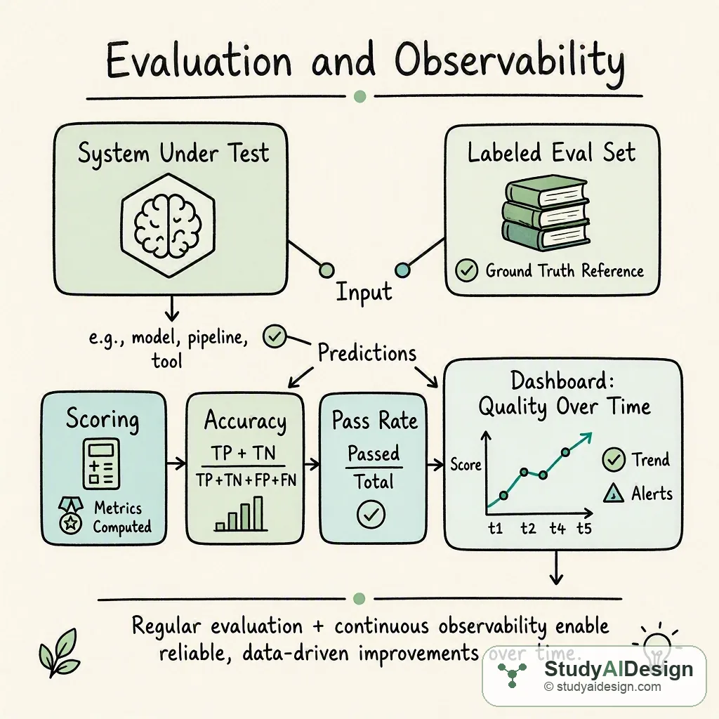
Building a language model application is only half the job. The other half is knowing whether it works. That sounds straightforward until you try to write it down: what does "works" mean for a system that produces open-ended text, where two perfectly correct answers may share zero words in common, and where a response can be technically accurate but completely unhelpful? Traditional software has unit tests and code coverage. Traditional ML has accuracy and F1 on a held-out set. LLM systems need something different, and the gap between needing it and having it well is where most teams run into trouble in production.
TL;DR
- LLM evaluation is hard because output is open-ended, ground truth is ambiguous or multi-valid, and quality is multi-dimensional (correctness, helpfulness, tone, safety do not reduce to a single number).
- Offline evaluation runs a fixed curated dataset in CI to catch known regressions before deployment; online evaluation samples 2 to 5 percent of production traffic to measure real query distribution and catch silent degradation.
- Build eval sets by sampling real production traffic, not internal brainstorming; 100 examples from production logs outperform 500 internally written examples because they cover edge cases you did not anticipate.
- LLM-as-judge scoring uses a secondary model to rate responses on specific criteria (correctness, helpfulness, grounding); it scales to arbitrary eval set sizes but requires careful rubric design and threshold calibration.
Key tradeoffs: Offline evaluation catches regressions in minutes but misses production tail distribution; online evaluation covers real queries but has hours-to-days latency before statistical power surfaces regressions.
Why LLM Evaluation Is Hard
The Open-Ended Output Problem
A customer support classifier has two outputs: escalate or do not escalate. You can label every test example and compute exact accuracy. A customer support LLM assistant can produce millions of distinct responses to the same question, most of them defensible, some of them subtly wrong in ways that only surface when a customer acts on the advice and something breaks downstream.
The problem compounds because LLM output quality is multi-dimensional. A response can be factually accurate but poorly structured. It can be beautifully written but miss the actual question. It can answer the literal question while violating a tone policy that the product team cares about deeply. These dimensions do not reduce to a single number, and optimizing one often trades off against another.
There is also the reference problem. Most automated metrics from the NLP literature assume you have a reference answer to compare against. For tasks like summarization, you can write one. For open-ended tasks like "explain this concept to a beginner" or "help me debug this code," the space of valid responses is enormous and writing a single reference that captures it is artificial. Comparing against a narrow reference penalizes correct responses that happen to use different words.
What Separates LLM Evaluation from Traditional ML
| Dimension | Traditional ML | LLM Systems |
|---|---|---|
| Output space | Finite classes or bounded numbers | Open-ended text |
| Ground truth | Clear and labelable | Often ambiguous or multi-valid |
| Metric | Accuracy, F1, RMSE | Composite scores, human preference |
| Automation | Fully automatable | Partial automation with human-in-loop |
| Regression | Easy (metric moves or not) | Subtle (quality shifts without hard breaks) |
| Latency of signal | Instant on test set | Delayed (need sampling + judging) |
The most important implication: you cannot evaluate an LLM system once at deployment and call it done. The model provider may silently update weights. Your prompt may start interacting differently with edge cases in production data. A new batch of users may bring query patterns you never anticipated. Evaluation needs to run continuously, not just at release time.
Offline vs Online Evaluation
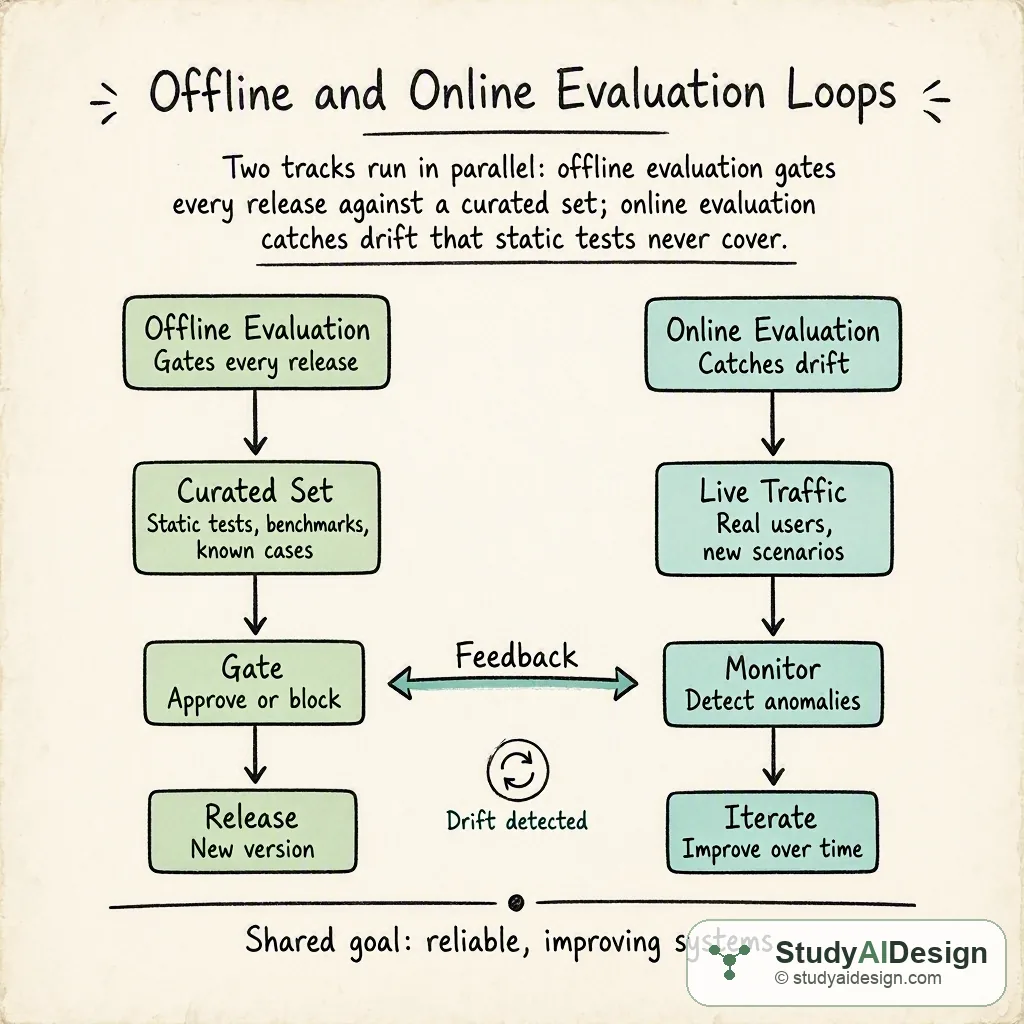
The single most useful structural distinction in LLM evaluation is offline versus online. They answer different questions and fail differently.
Offline Evaluation
Offline evaluation runs your system against a fixed, curated dataset before any user sees the output. You assemble a test set, run every example through the current system, score the results, and compare against a baseline or threshold. If the score falls below a threshold, you do not ship.
The strengths are control and repeatability. Every run uses the same inputs so you can attribute score changes to system changes. You can run it in CI and block deployments automatically.
The weakness is coverage. Your test set was written by you, or by a small team, representing the queries you thought to include. Production traffic will contain queries you never imagined: ambiguous phrasings, rare domains, adversarial edge cases, multilingual requests from users in countries you did not prioritize. A system with 90% quality on your eval set can have 60% quality on the long tail of production traffic.
Online Evaluation
Online evaluation measures quality on real production traffic. Since you cannot manually review every response, the standard approach is statistical sampling: evaluate a random 2 to 5% of live requests using an automated judge and aggregate the scores over time. Watch the aggregate trend, not any individual response.
The strengths are coverage and realism. You are measuring the actual distribution of user intent, not a curated approximation. Regressions that are invisible on your test set often surface quickly in online metrics because they affect the queries users actually send.
The weakness is latency. A quality regression that ships today might take hours or days to show up in sampled online metrics with enough statistical power to distinguish signal from noise. Offline evaluation catches known regressions in minutes.
Choosing the Right Mix
Both are necessary. The practical operating model for most teams:
- Offline gate: run on every pull request that touches prompts, retrieval, model config, or system architecture. Block the merge if any regression metric drops by more than a configured threshold (typically 3 to 5 percentage points relative to the previous release baseline).
- Online monitoring: sample 2 to 5% of production traffic continuously. Alert when a rolling 4-hour window drops more than 10% below the established baseline. This catches prompt degradation from silent model updates and distributional shifts that no test set predicted.
Building an Evaluation Set
What Goes in a Good Eval Set
A useful evaluation set has three properties: it is representative, it has ground truth (or a judging strategy), and it is adversarially diverse.
Representative means the query distribution matches production. If 60% of your production queries are short factual lookups and your eval set is 80% long analytical questions, your offline metrics are measuring a different product than the one users experience. Build your eval set by sampling real production traffic, not by brainstorming in a room.
Ground truth can take different forms depending on the task. For factual Q&A, it is a reference answer. For RAG, it is the set of documents that should be retrieved and a reference final answer. For summarization, it might be a set of required key points rather than a single reference. For open-ended tasks, ground truth is a judging rubric rather than a reference string.
Adversarial diversity means including the hard cases: queries that are ambiguous, queries that span multiple categories, queries designed to elicit hallucination, queries that test boundary conditions in your system prompt. These cases are disproportionately informative. A system that scores 95% on easy examples and 40% on adversarial ones is not a 90% system; it is a system with a known fragile region.
A Worked Example with Numbers
Consider a customer support assistant for a SaaS company. The team samples 500 real support tickets from the past three months, stratified across:
- 200 billing questions (reference answers derived from the billing policy document)
- 150 technical troubleshooting questions (reference answers verified by engineers)
- 100 feature availability questions (reference answers from the product changelog)
- 50 adversarial or ambiguous tickets (curated by the QA team)
They run the current system on all 500 and use LLM-as-judge scoring on four criteria (correctness, helpfulness, tone compliance, safety), each rated 1 to 5. Baseline scores before launch:
| Category | Correctness | Helpfulness | Tone | Safety |
|---|---|---|---|---|
| Billing (200) | 4.2 | 4.1 | 4.6 | 5.0 |
| Technical (150) | 3.8 | 3.9 | 4.5 | 5.0 |
| Feature (100) | 4.4 | 4.3 | 4.6 | 5.0 |
| Adversarial (50) | 2.9 | 3.1 | 4.2 | 4.7 |
The adversarial category scores lower across the board. The team investigates, discovers the model is hallucinating feature availability for sunset products, and adds a retrieval step specifically for the changelog. Adversarial correctness rises to 3.8 before launch. They now have a meaningful regression baseline: any future deployment that drops adversarial correctness below 3.5 gets blocked.
Reference-Based Metrics vs LLM as a Judge
Reference-Based Metrics
Reference-based metrics compare the model output to a gold-standard reference answer using automatic scoring functions.
ROUGE (Recall-Oriented Understudy for Gisting Evaluation) counts n-gram overlap between the prediction and the reference. ROUGE-1 is unigram overlap, ROUGE-2 is bigram overlap, ROUGE-L is longest common subsequence. Originally developed for summarization, ROUGE is fast and requires no external model calls. Its limitation is that it rewards lexical similarity, not semantic accuracy. A response that uses synonyms and paraphrases throughout can be factually identical to the reference and score poorly on ROUGE.
BERTScore addresses this by computing cosine similarity between BERT embeddings of prediction and reference tokens, allowing semantic matching across paraphrases. It correlates better with human judgment than ROUGE on most tasks but is still sensitive to reference quality and fails when the correct answer genuinely requires different vocabulary than the reference uses.
Exact match is the right tool for constrained extraction tasks: entity extraction, multiple-choice answers, short factual lookups where the answer is a date, a number, or a proper noun. When the correct answer space is this small, do not use a learned metric; just check equality.
LLM as a Judge
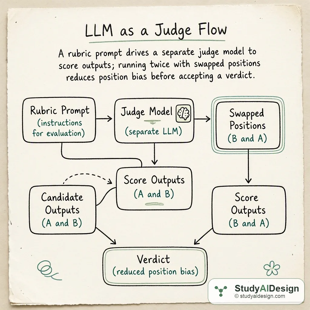
LLM-as-judge uses a separate language model to score outputs against a rubric. The judge model receives the query, the response, and optionally a reference answer, and returns a score with a brief justification. This approach generalizes to open-ended tasks where reference-based metrics fail.
A minimal judge prompt:
JUDGE_PROMPT = """
You are evaluating an AI assistant's response.
Question: {question}
Response to evaluate: {response}
Reference answer (if available): {reference}
Rate the response on the following criteria, each on a 1-5 scale:
- correctness: Is the factual content accurate?
- relevance: Does the response address the question asked?
- completeness: Are all key aspects covered without important omissions?
- helpfulness: Would a user find this genuinely useful?
Return a JSON object with keys: correctness, relevance, completeness, helpfulness, overall.
For each key, provide: {{"score": <int>, "reason": "<one sentence>"}}
"""The judge approach scales to any output type and produces human-readable justifications alongside scores, which is valuable for debugging regressions. The cost per evaluation is a full LLM inference call, so most teams run judges on 2 to 5% samples in production and on the full eval set in CI.
Tradeoffs
| Approach | Strengths | Weaknesses | Best for |
|---|---|---|---|
| Exact match | Zero cost, perfectly reproducible | Breaks on paraphrase | Short factual answers, classification |
| ROUGE | Fast, no API calls | Lexical; misses semantics | Summarization similarity |
| BERTScore | Semantic matching | Reference-dependent | Paraphrase detection |
| LLM judge (absolute) | Generalizes, human-readable | Costs inference per call, judge biases | Open-ended tasks |
| LLM judge (pairwise) | Strong for A/B comparisons | 2x cost; position bias | Model comparisons |
RAG-Specific Metrics
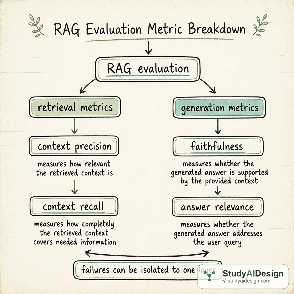
RAG systems have a unique evaluation structure because there are two distinct failure modes: bad retrieval and bad generation. Measuring only the final answer quality hides which layer is broken and makes it impossible to know where to spend optimization effort.
Context Recall
Context recall measures whether the retrieved chunks contain the information needed to answer the question. Formally: of all the factual claims in the ground-truth answer, what fraction are supported by at least one retrieved chunk?
A context recall of 0.60 means 40% of the ground truth claims are simply missing from the context window before the model even starts generating. No amount of generation-layer tuning can fix that; the fix is in retrieval.
Practically, context recall is measured by comparing each sentence of the reference answer against the pool of retrieved chunks using an LLM judge. If the judge determines a reference sentence is not entailed by any chunk, that sentence contributes to the numerator of a miss count.
Context Precision
Context precision measures whether the retrieved chunks are actually relevant to the query. A system that retrieves 10 chunks, 3 of which are relevant, has context precision of 0.30. Low precision means the LLM is reading mostly noise before generating, which increases token costs and dilutes the signal of relevant content.
Precision and recall trade off against each other at a given top-K cutoff. Increasing K from 5 to 10 typically improves recall (more chances to include the right chunk) but decreases precision (more noise enters the context). A reranker helps by reordering so that the most relevant chunks float to the top.
Faithfulness
Faithfulness measures whether the generated answer contains claims that are supported by the retrieved context. This is the metric most directly correlated with hallucination in a RAG system.
The measurement approach: decompose the generated answer into individual factual claims, then for each claim ask a judge model whether that claim is entailed by the retrieved context. Faithfulness = supported claims / total claims.
A faithfulness score of 0.85 means 15% of the generated claims have no support in the retrieved context. Some of these will be correct (the model happens to know the fact from training), but you cannot verify that, and a deployed system should not make claims it cannot attribute to its context.
Answer Relevance
Answer relevance measures whether the generated response actually addresses the user's question. A response can be faithful (every claim supported by the context) while being completely off-topic (the model answered a related but different question than the one asked). Relevance is typically measured by embedding the question and the answer and computing cosine similarity, or by asking a judge model whether the answer addresses the user intent.
Worked Example with Numbers
A technical documentation assistant, evaluated on a held-out set of 300 questions with labeled relevant documents:
| Pipeline configuration | Context recall | Context precision | Faithfulness | Answer relevance |
|---|---|---|---|---|
| Dense retrieval, top 10 | 0.64 | 0.48 | 0.78 | 0.82 |
| Hybrid (BM25 + dense), top 10 | 0.79 | 0.51 | 0.83 | 0.86 |
| Hybrid + reranker, top 5 | 0.77 | 0.74 | 0.91 | 0.89 |
Adding the reranker slightly reduced recall (top 5 vs top 10 means one fewer chance to include a needed chunk) but lifted precision dramatically (from 0.51 to 0.74) and faithfulness accordingly (from 0.83 to 0.91). The model was generating fewer hallucinated claims because the context window contained denser, more relevant content. The 2% recall drop was acceptable given the 8-point faithfulness gain.
Agent and Task Success Metrics
Agents introduce evaluation complexity that RAG pipelines do not have: multiple steps, multiple tool calls, and success criteria that are defined at the task level, not the response level.
Task Completion Rate
For a well-defined agentic task, define a binary or graded completion criterion that can be checked programmatically or by a judge after the full trajectory. A calendar scheduling agent either successfully created a meeting with all required participants in the correct time slot or it did not. A coding agent either produced code that passes the test suite or it did not.
Task completion rate is the fraction of test cases where the agent achieved the defined goal. Measure it on a curated set of representative tasks, not just the happy path. Intentionally include tasks that require error recovery (the first API call fails), tasks that require more steps than expected, and tasks with ambiguous instructions.
Tool Use Accuracy
For agents with access to multiple tools, track whether the agent selected the correct tool for each step and whether the tool call arguments were correct. Tool selection errors are often more diagnosable than final output errors because they are discrete: "used search instead of calendar API" is a more actionable signal than "output was unsatisfactory."
A useful breakdown: tool selection accuracy (did the agent call the right tool?), argument accuracy (were the arguments correctly extracted from context?), and tool result integration (did the agent correctly incorporate the tool's output into its next step?).
Multi-Turn Coherence
Evaluate whether the agent maintains consistent context across a multi-turn conversation. A customer support agent that forgets the account number a user provided three messages ago is failing a multi-turn coherence test. Build test cases that include references to earlier turns and verify the agent uses them correctly.
Human Evaluation
When Human Judgment Is Irreplaceable
Automated metrics, including LLM judges, are proxies for human judgment. They are calibrated against human labels during development, but the further a deployment drifts from the calibration distribution, the less the proxy tracks the thing you care about. Human evaluation is the ground truth.
Use humans when:
- Launching a new product category where you have no calibrated automated metrics
- Investigating a quality regression that automated metrics did not fully explain
- Evaluating safety, tone, and brand voice, where LLM judges have weaker agreement with human raters
- Running a final quality gate before a high-stakes deployment
Annotation Design
Annotation quality depends heavily on task definition. Raters who are asked to score "helpfulness from 1 to 5" without examples will produce inconsistent results. Design annotation tasks around clear criteria with calibration examples at each scale point.
A minimal annotation instruction for a support assistant:
- 5: Fully correct, addresses the exact question, tone is appropriate, no caveats needed
- 4: Correct with minor omissions or a slightly suboptimal phrasing
- 3: Partially correct; answers the literal question but misses a key nuance the user needed
- 2: Substantially incorrect or unhelpful; would mislead the user
- 1: Wrong, harmful, or completely off-topic
Start every annotation batch with 10 calibration examples that every rater sees and discusses before scoring the main batch. This anchors scale usage across raters.
Inter-Annotator Agreement
Before trusting human scores, measure inter-annotator agreement on a shared subset of 50 to 100 examples. The standard metric is Cohen's Kappa, which corrects for chance agreement. Kappa below 0.40 indicates poor alignment (either the task is poorly defined, the calibration set is inadequate, or the raters need more training). Kappa above 0.60 is a reasonable target for nuanced quality ratings. For binary safety labels, target above 0.75.
Regression Testing and CI for Prompts
Prompts are code. Changing a prompt is a code change. Deploying a prompt change without running a regression test is equivalent to merging a function change without running the test suite.
Building a Regression Test Suite
A prompt regression suite needs at minimum:
- A representative sample of queries (100 to 500) with recorded expected behavior (not necessarily exact string matches, but behavioral assertions)
- A baseline run against the current production prompt, stored with timestamps
- A diff mechanism that computes score changes between the candidate and baseline
Behavioral assertions are more robust than string matching. Instead of "response must contain the phrase 'contact support'," use "response must not suggest a workaround that requires admin privileges" or "response must address the billing question without mentioning unrelated product features." These assertions can be evaluated by a judge model or by a lightweight classifier.
Integrating into CI
The practical integration pattern:
# .github/workflows/eval.yml (example structure)
on:
pull_request:
paths:
- 'prompts/**'
- 'config/model*.yaml'
- 'retrieval/**'
jobs:
eval:
runs-on: ubuntu-latest
steps:
- name: Run offline eval
run: python evals/run_eval.py --compare-baseline --threshold 0.03
- name: Comment results on PR
uses: actions/github-script@v6
# posts score table as a PR commentThe --threshold 0.03 flag means: block the PR if any tracked metric drops more than 3 percentage points relative to the baseline. Post the full score table as a PR comment so reviewers can see the tradeoffs.
Blocking vs Warning Thresholds
Not every regression should block deployment. A useful two-tier system:
- Block: core quality metrics (correctness, faithfulness, safety) drop more than the configured threshold. Require explicit override approval.
- Warn: secondary metrics (response conciseness, format compliance) drop. Post a warning but allow the merge. Document the drift.
Teams that start with blocking on everything and then turn off the gate after the first inconvenient failure learn nothing. Calibrate the thresholds against historical change impact before enforcing them.
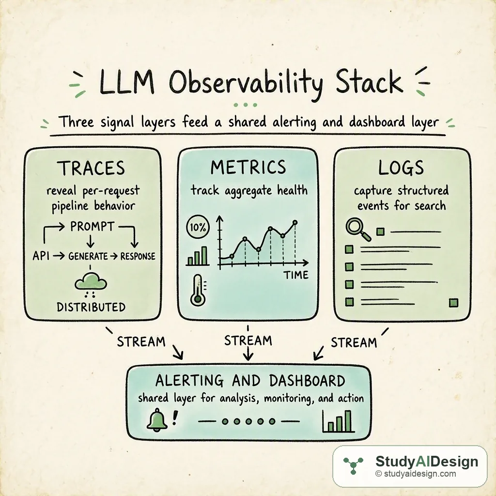
Observability: Tracing, Logging, Cost and Latency
Running evaluation offline and during CI catches planned regressions. Observability catches everything else: silent model provider updates, prompt drift under real traffic distribution, cost anomalies, and tail-latency spikes that only surface under load.
Distributed Tracing
An LLM pipeline is a multi-step operation. A RAG query involves an embedding call, a vector search, potentially a reranker inference call, and a generation call. Without tracing, when a request takes 4 seconds you cannot tell whether 3.5 of those seconds came from vector search or from the LLM. Tracing attributes latency to components.
Instrument each pipeline step as a span using OpenTelemetry or an LLM-native tracing library (Langfuse, LangSmith, Arize Phoenix). Every span should record:
with tracer.start_span("retrieval") as span:
span.set_attribute("query_length_tokens", len(tokens))
results = vector_db.search(embedding, top_k=10)
span.set_attribute("results_returned", len(results))
span.set_attribute("top_score", results[0].score if results else 0)Group all spans from one user request under a single trace ID. This lets you pull the full waterfall for any request that a user reports as slow or wrong.
Structured Logging
Log every request with enough context to reproduce it. For LLM requests, the minimum log record:
- Timestamp and request ID
- Model name and version
- Input token count (not the raw content if you have privacy requirements)
- Output token count
- Time to first token and total latency
- A hash of the input content (for deduplication and privacy-preserving analysis)
- Application-level metadata: user tier, feature flag state, prompt version ID
Avoid logging raw user content unless your data handling agreements explicitly permit it. Hashing content lets you correlate requests across logs without storing sensitive text.
Cost and Latency Monitoring
Cost is a first-class operational metric, not a billing afterthought. At scale, small inefficiencies compound:
# Track cost at request time
PRICING = {
"gpt-4o": {"input": 2.50, "output": 10.00}, # per 1M tokens
"gpt-4o-mini": {"input": 0.15, "output": 0.60},
}
def log_cost(model, input_tokens, output_tokens, request_id):
p = PRICING[model]
cost = (input_tokens / 1e6) * p["input"] + (output_tokens / 1e6) * p["output"]
metrics.increment("llm.cost_usd", cost, tags={"model": model})
metrics.increment("llm.tokens.input", input_tokens, tags={"model": model})
metrics.increment("llm.tokens.output", output_tokens, tags={"model": model})Alert when hourly cost exceeds 2x the rolling 7-day average at the same hour. This catches traffic spikes, accidental context size inflation from a bad prompt change, and runaway retry loops before they become a billing surprise.
For latency, track p50, p95, and p99 separately. p95 and p99 diverge from p50 for LLM calls because tail latency is driven by context length variation and provider queueing, not by base model speed. A system with p50 of 1.2 seconds and p99 of 12 seconds has a very different user experience story than one with p50 of 1.5 seconds and p99 of 2.5 seconds.
Failure Modes
Gaming the Metric
Once a metric is defined and tracked publicly, the system (or the team maintaining it) will optimize for the metric rather than the underlying quality it was meant to proxy. An LLM-as-judge score can be gamed by adding sycophantic filler text that flatters the judge model, by writing longer responses (length bias), or by using a system prompt that is specifically tuned to the judge model's preferences rather than to user needs.
The defense is to treat no single metric as the target, to hold out a small set of human-labeled examples that are never used during optimization and serve as a periodic ground truth audit, and to rotate the judge model periodically so that gaming the specific judge does not persist.
Judge Bias
Beyond position and length bias already covered, LLM judges show cultural and linguistic bias (preferring responses in formal standard English), confirmation bias (tending to rate responses that agree with prior claims in the rubric as more correct), and recency bias (favoring content near the end of a long context). These biases do not average out with more samples; they are systematic.
Concrete mitigation steps:
- Run a correlation audit between judge scores and response length on your current eval set. If the correlation is above 0.3, your judge is length-biased; add explicit anti-length instructions to the rubric.
- Use human labels as calibration anchors and check judge agreement against them monthly. If agreement drops, re-evaluate the judge model and rubric.
- For pairwise comparisons, always present both orderings (A-then-B and B-then-A) and filter out inconsistent verdicts. A consistent verdict with high confidence is more reliable than two verdicts that were the same by chance.
Evaluation Set Drift
Your eval set was representative when you built it. Six months later, product scope has expanded, the user base has shifted, and the query distribution in production looks different from the queries in your test file. An eval set that no longer reflects reality provides a false sense of security: you are passing a test of the product you used to have.
Schedule quarterly eval set reviews. Sample fresh production traffic, inspect it for new patterns, and add representative examples to the eval set. Archive old examples that no longer reflect the current product scope rather than letting them dilute the signal. Treat the eval set as a living artifact that requires maintenance, not a one-time artifact that requires storage.
Interview angle
Related Topics
How would you rate the quality of this article?
Keep going
Practice what you just read against real interview questions, or carry on through the curriculum.