inference optimization
Part of the AI system design curriculum
Inference Optimization
How LLM serving works under the hood, and the techniques that make it fast, cheap, and scalable in production.
TL;DR
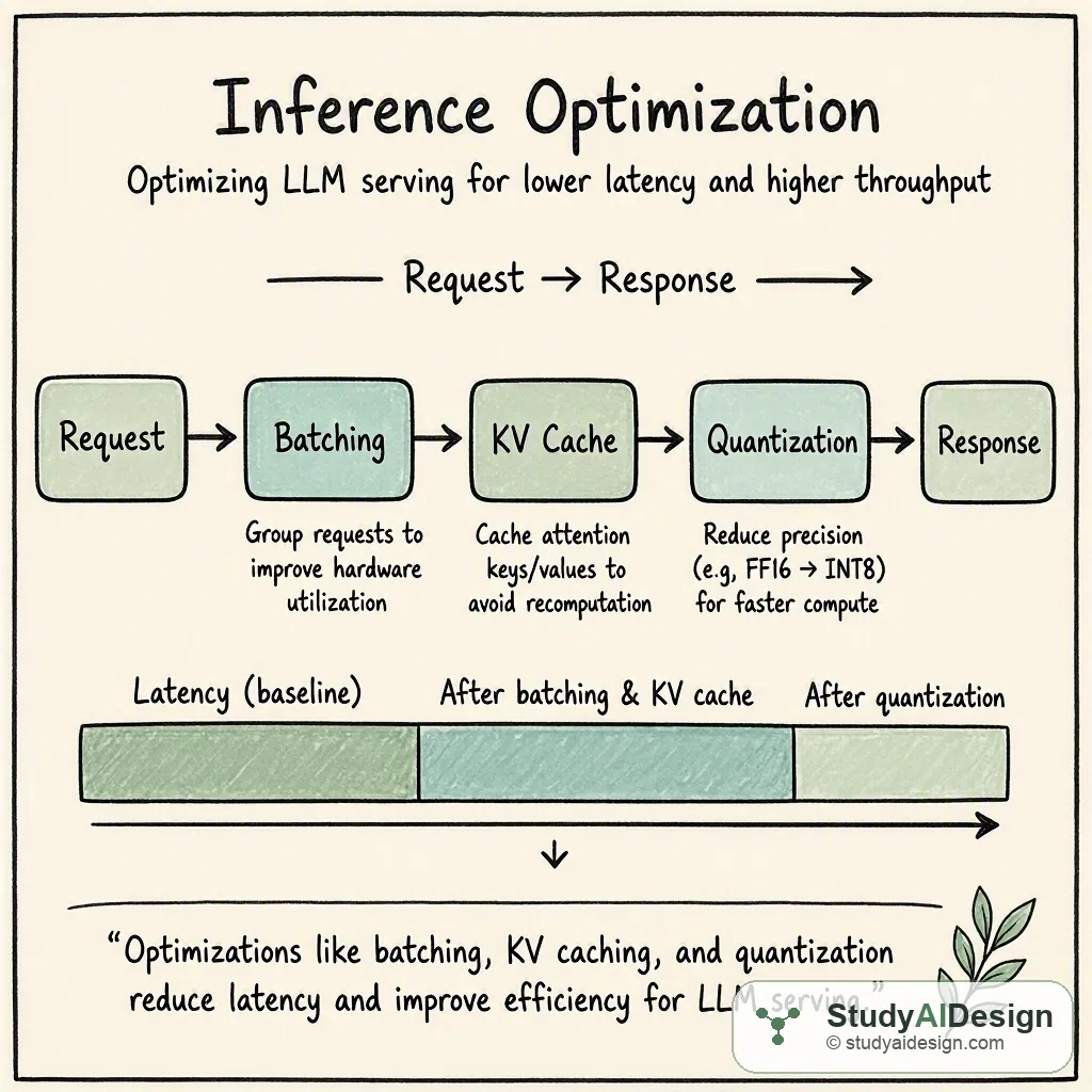
- Inference splits into two phases: prefill is compute bound and drives time to first token, while decode is memory bound and drives time per output token.
- The KV cache stores attention states to avoid recomputing them, making memory the binding constraint for serving long context workloads.
- Continuous batching and PagedAttention work together to minimize idle GPU time and memory fragmentation, often improving throughput by 4x to 10x.
- Quantization speeds up the decode phase by shrinking model weights, which reduces the amount of data moved across the memory bus per step.
- Speculative decoding uses a smaller draft model to predict multiple tokens at once, accelerating decode for low temperature or structured tasks.
When you deploy a language model, the training bill is already paid. Every dollar you spend from that point forward is inference cost: GPU time, memory, and bandwidth consumed as the model converts prompts into tokens. Getting inference right is not just about speed. It shapes what batch sizes your hardware can sustain, how many concurrent users you can serve, and whether the unit economics of your product hold up under real load. The techniques in this chapter address each of those concerns from first principles, starting with how the model actually computes a single token and ending with a worked example that shows what compounding four orthogonal optimizations can do to cost.
The Inference Cost Model
LLM inference splits into two fundamentally different computational phases. Each has a different bottleneck, and each responds to a different class of optimization. Understanding this split is the prerequisite for every technique that follows.
Prefill: Compute-Bound
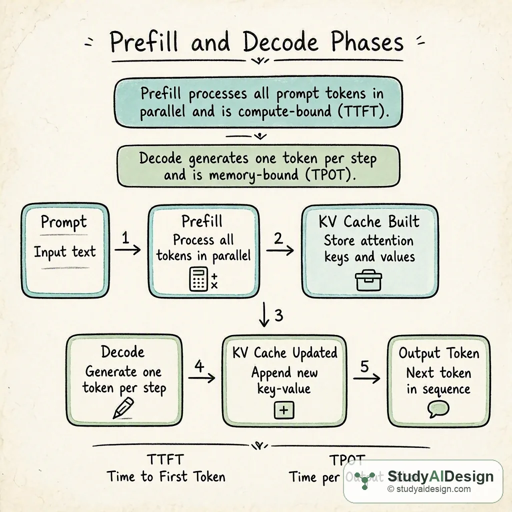
During prefill, the model processes every token in the input prompt simultaneously. Attention is computed over all positions in parallel, weight matrices are multiplied against a full matrix of activations, and the resulting Key and Value tensors are written into a cache for later use. This parallelism saturates the GPU's arithmetic units. Prefill is compute-bound: the limiting factor is the number of floating-point operations the hardware can execute per second.
For a 70B parameter model on an H100 with roughly 1,979 TFLOPS of BF16 throughput, prefilling a 4,096-token prompt takes around 80 milliseconds. That 80 ms is what the user perceives as initial response latency, which is why it maps directly to the Time to First Token (TTFT) metric.
Decode: Memory-Bound
Once the first token is generated, the decode phase begins. Tokens come out one at a time. Generating each new token requires loading the entire weight matrix from GPU memory, performing a matrix-vector multiply against the current hidden state, and appending new Key and Value entries to the cache. At every step you are moving roughly 140 gigabytes of weight data from VRAM to compute units in order to produce a single 2-byte output token. The throughput ceiling is the memory bus, not the arithmetic cores.
An H100 has 3.35 TB/s of HBM3 memory bandwidth. Transferring 140 GB takes about 42 ms, which is why a 70B model decodes at roughly 20 to 25 tokens per second per request in isolation. The GPU's arithmetic units are mostly idle during this transfer, waiting on data. Decode is memory-bound, and making it faster means reducing how much data moves on each step.
Key Metrics
Two user-visible metrics capture the effect of these phases:
- TTFT (Time to First Token): the delay between sending a request and receiving the first response token. Dominated by prefill time. Matters most for interactive applications where users feel the initial pause.
- TPOT (Time Per Output Token): the delay between successive generated tokens. Dominated by decode time. Matters for streaming responsiveness and reading speed.
Optimizing TTFT targets the prefill path: use FlashAttention to reduce memory reads during the quadratic attention computation, increase tensor parallelism to run larger matrix multiplies across more GPUs, or skip prefill entirely with prefix caching for requests that share a common prompt prefix. Optimizing TPOT targets the decode path: quantize weights to move fewer bytes per step, use grouped-query attention to shrink the KV cache so more requests fit per batch, or apply speculative decoding to generate multiple tokens per memory load.
The KV Cache and Its Memory Cost
Every token generated during decode depends on the attention keys and values of all preceding tokens. Recomputing them from scratch on every step would be prohibitively slow, so the model maintains a KV cache that stores these tensors across the sequence. The cache eliminates redundant computation at the direct cost of GPU memory.
Memory Math
The KV cache size for a single request is:
KV bytes = 2 (K and V)
x num_layers
x context_length
x num_kv_heads
x head_dim
x bytes_per_element
For Llama 3 70B with Grouped-Query Attention (8 KV heads) at BF16 precision:
2 x 80 x 128,000 x 8 x 128 x 2 = roughly 42 GB per request at full 128k context
For a batch of four concurrent users at 128k context, the KV cache alone requires 168 GB, exceeding the 80 GB capacity of a single H100. Without GQA, with 64 KV heads (Multi-Head Attention), that figure climbs to roughly 336 GB per request - physically impossible on a single GPU at that context length.
Grouped-Query Attention
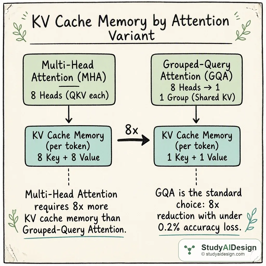
The KV cache grows proportionally to the number of KV heads. Multi-Head Attention (MHA) uses one KV head per query head, so a 64-query-head model allocates 64 KV head pairs per layer. Grouped-Query Attention (GQA) groups multiple query heads to share a single KV head pair. With 8 KV groups instead of 64, memory consumption drops eightfold with under 0.2% accuracy loss on standard benchmarks. All production-scale models released after 2023 ship with GQA by default. Multi-Query Attention (MQA) is the extreme case: one KV head shared across all query heads, reducing memory 64x but at a 2 to 3% accuracy penalty.
Context Caching
When many requests share a common prefix (a 10,000-token system prompt, a shared knowledge base, or a fixed tool schema), the KV tensors for that prefix need only be computed once and can be reused across every request that shares it. All major API providers expose this as prompt caching, with input token discounts ranging from 50% (OpenAI) to 90% (Anthropic). On self-hosted systems, frameworks like SGLang implement tiered caching: the most recent KV blocks stay in VRAM, frequently accessed blocks spill to CPU RAM, and cold prefixes live on SSD with access latency in the tens of milliseconds rather than hundreds.
The economics require a break-even calculation. Anthropic writes a 25% premium on cached tokens, so a prefix must be reused at least 1.3 to 1.5 times before caching saves money. For a shared system prompt that thousands of requests use daily, the savings are large. For a unique long context per user session, caching provides no benefit.
Batching Strategies
A single request during decode uses a tiny fraction of GPU compute because each decode step is a matrix-vector multiply rather than a matrix-matrix multiply. The GPU wants many requests running simultaneously so it can combine those per-request vector operations into batched matrix operations that actually saturate its arithmetic units.
Static vs. Continuous Batching
Traditional ML serving uses static batching: requests are grouped at submission time, processed together, and released together. The GPU waits for the entire batch to finish before accepting new work. For variable-length LLM generation, this forces every request to wait for the longest-generating request in the batch. A batch where one request produces 500 tokens and the others produce 10 tokens each wastes 97% of the batch's remaining GPU time sitting idle on those short requests while the long one finishes.
Continuous batching, introduced in the Orca paper and widely deployed through vLLM, makes the scheduling decision at the level of individual token generation steps rather than at the request level. When a request completes its last token, its KV cache memory is freed immediately and a new request from the queue fills that slot on the very next decode iteration. The batch composition changes every step. GPU utilization stays high because there are no forced idle periods.
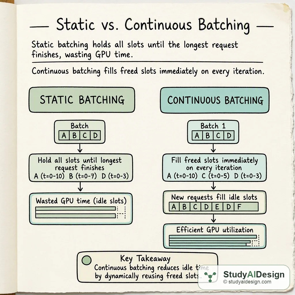
For workloads where output lengths vary by a factor of 10 or more (typical in chat applications), continuous batching typically improves aggregate throughput by 4x to 10x compared to static batching.
Chunked Prefill
A single long-context prefill can monopolize the GPU for two to three seconds, causing decode latency to spike sharply for all other in-flight requests. This is called a prefill stall, and it shows up as a dramatic spike in p99 TPOT without any corresponding change in median TPOT.
Chunked prefill fixes this by breaking the long prefill into segments of a few thousand tokens each, interleaved with regular decode iterations. Each chunk takes on the order of 80 ms. Between chunks, the engine runs one decode step for all in-flight requests. The user with the long prompt sees a slightly higher TTFT; all other users maintain smooth TPOT throughout.
Speculative Decoding
The core inefficiency of decode is that each memory-bound step produces only one token. Speculative decoding exploits the observation that a small model can cheaply predict the next K tokens, and a large model can verify all K predictions simultaneously in a single parallel forward pass.
The Draft-Verify Loop
- A small draft model (1B parameters, roughly 5 ms per token) generates K candidate tokens sequentially.
- The large target model (70B parameters, roughly 50 ms per forward pass) processes all K draft tokens at once in a prefill-style parallel pass.
- The target model's output distribution at each position is compared against the draft token using a rejection sampling criterion. If the distributions match closely enough, the token is accepted. The first rejected token, call it position i, causes all subsequent draft tokens (positions i+1 through K) to be discarded.
- When all K tokens are accepted, the sequence has advanced K positions in roughly the same wall-clock time that a single standard decode step would have taken.
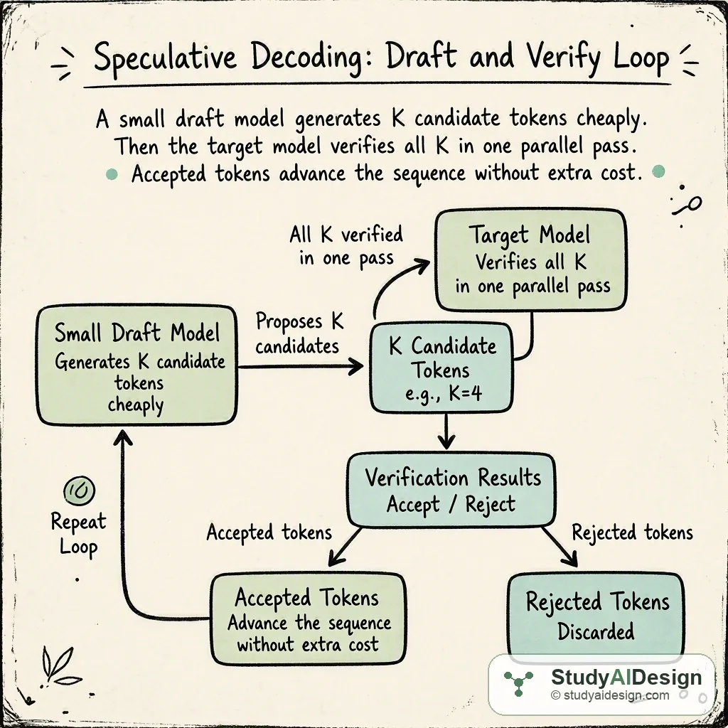
The net speedup depends on the acceptance rate. For greedy or low-temperature generation on structured tasks (code completion, structured extraction, summarization), acceptance rates of 80 to 90% are typical, yielding 2x to 3x end-to-end speedup. For high-temperature creative generation where the probability distribution is flat, the draft model's predictions are frequently wrong, acceptance rates fall below 50%, and the overhead of running the draft model can make the system slower than standard decoding.
Medusa heads eliminate the need for a separate draft model. Instead of a second 1B model consuming additional VRAM, a set of small linear layers is attached to the final hidden state of the target model, each head trained to predict tokens at a different future offset. All predictions are produced within a single forward pass of the target model, with no second model, no inter-model communication, and no additional KV cache. The trade-off is that Medusa heads require a fine-tuning step to train.
PagedAttention and vLLM
Before vLLM, most serving systems pre-allocated a contiguous block of GPU memory per request sized to the maximum possible output length. A request that generated 50 tokens instead of the reserved 2,048 left 97.5% of its allocation sitting empty throughout its lifetime. Combined with the external fragmentation that accumulates between allocations, GPU memory utilization in practice stayed at 60 to 70% under load.
PagedAttention (Kwon et al., SOSP 2023) applies the virtual memory model from operating systems. The KV cache is divided into fixed-size blocks of 16 tokens each. Each request maintains a block table that maps logical block indices to physical VRAM addresses scattered throughout the device. Blocks are allocated only when tokens arrive, not speculatively to the maximum length. When a request finishes, its blocks return to the free pool immediately.
Under production load, this drops memory waste below 4%. That efficiency gain compounds: more concurrent requests fit in the same VRAM, which increases batch sizes, which converts per-request decode steps from matrix-vector back toward matrix-matrix operations, which raises arithmetic unit utilization and aggregate throughput.
PagedAttention also enables prefix sharing at zero copy cost. When 100 requests share a 5,000-token system prompt, the KV blocks for that prefix are allocated once, and each request's block table simply points to the same physical blocks. Copy-on-write semantics handle divergence: the first unique token a request generates triggers allocation of a new block, leaving the shared blocks untouched.
Quantization for Serving
Model weights are the primary source of memory bandwidth consumption during decode. A 70B BF16 model requires moving 140 GB per decode step. Quantizing to 8-bit integers halves this to 70 GB; quantizing to 4-bit reduces it to 35 GB. Halving the data moved roughly doubles decode throughput.
Modern inference prefers FP8 (8-bit floating point) over INT8 for activations because FP8 retains more of the dynamic range that attention mechanisms need. H100 and B200 GPUs have native FP8 tensor cores, making FP8 essentially free in terms of implementation complexity: the serving framework sets a flag and the hardware handles the rest.
The tension is always accuracy versus compression. INT4 quantization (via GPTQ or AWQ) degrades standard benchmark scores by 1 to 3% and shows larger gaps on tasks requiring precise recall of numerical facts or exact string matching. The right level of quantization depends on what your application can tolerate.
| Quantization | Weight bits | Memory vs BF16 | Decode speedup | Typical accuracy loss |
|---|---|---|---|---|
| BF16 (baseline) | 16 | 1x | 1x | 0% |
| FP8 | 8 | 0.5x | roughly 2x | under 0.1% |
| INT8 (AWQ) | 8 | 0.5x | roughly 2x | 0.2 to 0.5% |
| INT4 (GPTQ) | 4 | 0.25x | roughly 3x to 4x | 1 to 3% |
| INT4 (AWQ) | 4 | 0.25x | roughly 3x to 4x | 0.5 to 1.5% |
Throughput, Latency, and Cost Tradeoffs
Every optimization in this chapter involves a tradeoff. Understanding the structure of those tradeoffs is what separates a system that performs well in benchmarks from one that meets real user requirements.
The Throughput-Latency Curve
Adding requests to a batch increases aggregate throughput (total tokens per second across all requests) but also increases per-request latency, because each decode step now involves more computation. At low batch sizes, the GPU is underutilized and throughput scales nearly linearly with batch size at almost no latency cost. Above a saturation point, adding more requests increases latency without proportionally improving throughput. The optimal operating point is workload-specific: streaming chat applications want low TPOT at the cost of lower peak throughput; batch analytics jobs want maximum throughput at the cost of higher latency per item.
Technique Selection Guide
| Technique | Primary gain | Secondary cost | When to reach for it |
|---|---|---|---|
| Continuous batching | Throughput 4x to 10x | Slight latency variance | Always, for any production LLM serving |
| PagedAttention | Memory utilization above 96% | None at inference time | Default in vLLM and SGLang; use these frameworks |
| KV cache quantization | Memory 2x to 4x | Negligible accuracy impact | Long contexts, many concurrent users |
| Grouped-Query Attention | KV cache 8x smaller | Requires model to be trained with GQA | Use models already trained with GQA |
| Speculative decoding | Latency 2x to 3x | Adds VRAM for draft model; degrades at high temperature | Low-temperature structured generation |
| INT4 quantization | Decode throughput 3x to 4x | 1 to 3% accuracy loss | High-throughput serving with acceptable quality tradeoff |
| Chunked prefill | Stable p99 TPOT | Slightly higher TTFT for long prompts | Mixed short-and-long-context workloads |
| Prefix caching | TTFT near zero on cached portion | Storage overhead | Shared system prompts, multi-turn chat |
Worked Example: Compounding Optimizations on a Single H100
Consider a customer support application generating 10 million output tokens per day, running a 70B model on a single H100 (80 GB VRAM, 3.35 TB/s memory bandwidth).
Baseline: static batching, BF16, no optimizations
Decode throughput per request: roughly 25 tokens/second. Memory per request KV cache at 4k context: roughly 5 GB. With 80 GB VRAM and 140 GB of weights (needing to share across pipeline stages, practically fitting in 40 GB for weights with memory reuse), batch size tops out at about 4 requests.
- Aggregate throughput: 4 x 25 = 100 tokens/second
- Time to process 10M tokens: 28 hours (cannot keep up with a 24-hour window)
- Cost at 2.50 per million output tokens
After continuous batching + PagedAttention
Memory fragmentation drops below 4%, allowing batch size to grow from 4 to around 20 requests without any additional VRAM.
- Aggregate throughput: 20 x 25 = 500 tokens/second
- Time for 10M tokens: 5.5 hours, fits within the day
- Cost per million output tokens: roughly $0.50
After adding FP8 quantization
Weight data moved per decode step drops from 140 GB to 70 GB. Decode throughput per request roughly doubles.
- Decode throughput: roughly 50 tokens/second per request
- Aggregate at batch 20: roughly 1,000 tokens/second
- Cost per million output tokens: roughly $0.25
After adding speculative decoding (1B draft model, 80% acceptance rate at low temperature)
Effective tokens produced per wall-clock second roughly doubles again.
- Effective throughput: roughly 2,000 tokens/second
- Cost per million output tokens: roughly $0.12
- Total improvement vs. baseline: roughly 20x cost reduction
The key insight is that each optimization targets a different bottleneck. Continuous batching and PagedAttention address GPU utilization and memory fragmentation. FP8 addresses memory bandwidth. Speculative decoding addresses the serial structure of the decode loop. Because these are orthogonal, their effects compound rather than overlap.
Interview angle
Related Topics
How would you rate the quality of this article?
Keep going
Practice what you just read against real interview questions, or carry on through the curriculum.